U²-Net and BASNet: Nested Architectures and Boundary-Aware Training

March 29, 2026

U²-Net and BASNet: Nested Architectures and Boundary-Aware Training

Target audience: ML practitioners familiar with encoder-decoder architectures (U-Net, ResNet) who want to understand two key innovations in salient object detection: how to build deeper multi-scale architectures without pretrained backbones, and how to train and evaluate models that produce sharp, accurate boundaries.

---

Table of Contents

1. Overview
2. U²-Net: The RSU Block
3. U²-Net: Full Architecture
4. BASNet: The Hybrid Loss
5. BASNet: Relaxed Boundary F-measure
6. Summary
7. Key References

---

Overview

Standard U-Net architectures use plain convolutional blocks (residual blocks, dense blocks, or inception modules) at each encoder-decoder stage. These blocks extract features at a single scale per stage – multi-scale fusion only happens across stages through the skip connections. This limits how rich the features are at any given stage, and typically requires a heavy pretrained backbone (VGG-16, ResNet-50) to compensate.

U²-Net (Qin et al., 2020) solves this by replacing each plain block with a ReSidual U-block (RSU) – a miniature U-Net that captures multi-scale context within each stage. This “U-structure within U-structure” design enables training from scratch on small datasets while matching or exceeding methods that rely on ImageNet-pretrained backbones.

BASNet (Qin et al., CVPR 2019) tackles a different but complementary problem: how to train and evaluate boundary quality. Most saliency methods optimize cross-entropy, which treats all pixels equally and produces blurry boundaries. BASNet introduces a hybrid loss fusing BCE, SSIM, and IoU to supervise at pixel, patch, and map levels simultaneously. It also adopts the relaxed boundary F-measure to quantitatively evaluate boundary accuracy – a metric that standard region-based metrics miss entirely.

We start with U²-Net’s core innovation – the RSU block – then zoom out to the full architecture, before turning to BASNet’s training and evaluation contributions.

---

1. The RSU Block: A U-Net Inside a U-Net

The core building block of U²-Net is the ReSidual U-block (RSU). Instead of stacking a few convolutions at each encoder-decoder stage, the RSU block runs a complete internal encoder-decoder, giving each stage its own multi-scale feature extraction pipeline.

RSU-L: The Standard Block

An RSU-L block has three parameters: $L$ (depth of the internal U-structure), $C_{in}$/$C_{out}$ (input/output channels), and $M$ (channels in all internal layers). It works in three steps:

1. Input transform: A single $3 \times 3$ Conv + BatchNorm + ReLU maps the input to $C_{out}$ channels, producing a feature map $\mathcal{F}(x)$
2. Internal U-structure: An $L$-level symmetric encoder-decoder:
   • Encoder: $L$ layers of Conv+BN+ReLU (each with $M$ channels), with MaxPool between layers to halve the resolution at each level
   • Bottleneck: A dilated convolution (dilation=2) at the deepest level
   • Decoder: $L$ layers of Conv+BN+ReLU with bilinear upsampling, plus skip connections (concatenation) from the corresponding encoder level
3. Residual fusion: The internal U-structure output is added element-wise to $\mathcal{F}(x)$

The key insight is that pooling inside the RSU block means most internal computation happens on downsampled feature maps. An RSU-7 block has 7 internal encoder levels, but the convolutions at deeper levels operate on $\frac{1}{64}\times$ resolution feature maps – making it computationally cheap to go deep.

RSU-LF: The Dilated Variant

At deeper stages of the outer U-Net, feature maps are already small (20x20 or 10x10). Further pooling would destroy spatial information. The RSU-LF variant (“F” for flat) replaces all pooling and upsampling with dilated convolutions at increasing dilation rates:

• Encoder: dilation rates $1 \to 2 \to 4 \to 8$
• Decoder: dilation rates $4 \to 2 \to 1$, with skip connections

All internal feature maps maintain the same spatial resolution. RSU-4F still captures multi-scale context through the expanding receptive fields of the dilated convolutions, without any spatial downsampling.

With the RSU block defined, we can now see how U²-Net assembles these blocks into a complete encoder-decoder architecture.

---

2. U²-Net: Full Architecture

The complete U²-Net is a 6-stage encoder-decoder where every stage uses an RSU block. Input images are resized to $320 \times 320$.

Encoder Path

Stage	Block	Resolution	Output Channels	Internal Channels ($M$)
En_1	RSU-7	320x320	64	32
En_2	RSU-6	160x160	128	32
En_3	RSU-5	80x80	256	64
En_4	RSU-4	40x40	512	128
En_5	RSU-4F	20x20	512	256
En_6	RSU-4F	10x10	512	256

Between encoder stages, MaxPool with stride 2 halves the spatial resolution. Notice the pattern: shallower stages use deeper RSU blocks (RSU-7 at full resolution) because their large feature maps can support multiple rounds of internal pooling. Deeper stages switch to RSU-4F because their small feature maps cannot afford further downsampling.

Decoder Path

Stage	Block	Resolution	Output Channels	Internal Channels ($M$)
De_5	RSU-4F	20x20	512	256
De_4	RSU-4	40x40	256	128
De_3	RSU-5	80x80	128	64
De_2	RSU-6	160x160	64	32
De_1	RSU-7	320x320	64	16

Each decoder stage receives the concatenation of the upsampled output from the deeper stage and the skip connection from the corresponding encoder stage. This doubles the input channel count (e.g., De_5 receives $512 + 512 = 1024$ channels).

Deep Supervision

U²-Net generates a saliency prediction from every decoder stage plus the bottleneck, for a total of 6 side outputs:

1. Each stage (De_1 through De_5, plus En_6) produces a feature map
2. A $3 \times 3$ Conv reduces each to 1 channel
3. Bilinear upsampling brings each to the full $320 \times 320$ resolution
4. All 6 maps are concatenated and fused via a $1 \times 1$ Conv into the final prediction $d_0$
5. All 7 outputs ($d_0$ plus $d_1$ through $d_6$) pass through sigmoid activation

The training loss sums binary cross-entropy over all 7 outputs:

\[\mathcal{L} = \sum_{m=1}^{6} w_{side}^{(m)} \cdot \ell_{bce}^{(m)} + w_{fuse} \cdot \ell_{fuse}\]

• $\ell_{bce}^{(m)}$: BCE loss for the $m$-th side output
• $\ell_{fuse}$: BCE loss for the fused output $d_0$
• All weights $w$ are set to 1

Deep supervision forces each decoder stage to produce a meaningful saliency estimate independently, preventing vanishing gradients in deeper stages.

U²-Net vs U²-Net† (Lightweight Variant)

U²-Net† uses the same topology but drastically reduces channel counts: all encoder outputs are fixed at 64 channels, and all internal channels $M = 16$. This shrinks the model from 176 MB (~44M parameters) to just 4.7 MB (~1.1M parameters) while retaining competitive performance.

Model	Parameters	Size	FPS (GTX 1080Ti)
U²-Net	~44M	176 MB	30
U²-Net†	~1.1M	4.7 MB	40

The lightweight variant still outperforms many methods that use heavy pretrained backbones – a testament to the architectural efficiency of the nested U-structure. The paper generalizes this concept as U$^n$-Net: $n$ levels of nesting. U²-Net uses $n = 2$, and higher $n$ would nest further, though $n = 2$ already achieves state-of-the-art results.

U²-Net addresses the architecture question – how to extract rich multi-scale features. But architecture alone does not guarantee sharp boundaries. Next, we turn to BASNet’s contributions on the training and evaluation side.

---

3. BASNet: The Hybrid Loss

Most salient object detection methods train with Binary Cross-Entropy (BCE) alone. BCE compares each pixel independently against the ground truth – it treats boundary pixels and interior pixels with equal importance. This leads to a well-known problem: models trained with BCE produce blurry, uncertain boundaries because the loss provides weak gradient signal for boundary pixels that are inherently ambiguous.

BASNet addresses this by fusing three complementary losses that supervise at different spatial scales:

\[\ell^{(k)} = \ell_{bce}^{(k)} + \ell_{ssim}^{(k)} + \ell_{iou}^{(k)}\]

Each loss component captures a different level of structure.

Pixel Level: Binary Cross-Entropy

BCE is the standard pixel-wise classification loss:

\[\ell_{bce} = -\sum_{(r,c)} \left[ G(r,c) \log S(r,c) + (1 - G(r,c)) \log(1 - S(r,c)) \right]\]

• $G(r,c) \in {0, 1}$: ground truth label at pixel $(r, c)$
• $S(r,c)$: predicted probability of being salient

BCE provides a smooth gradient for all pixels and helps the network converge. But it does not consider neighborhood structure – a pixel’s loss is independent of its neighbors.

Patch Level: Structural Similarity (SSIM)

SSIM was originally designed for image quality assessment. It compares local patches between the prediction and ground truth, capturing structural patterns that pixel-wise metrics miss. Given two corresponding patches $\mathbf{x}$ and $\mathbf{y}$ (size $N \times N$, where BASNet uses $N = 11$) cropped from $S$ and $G$:

\[\ell_{ssim} = 1 - \frac{(2\mu_x \mu_y + C_1)(2\sigma_{xy} + C_2)}{(\mu_x^2 + \mu_y^2 + C_1)(\sigma_x^2 + \sigma_y^2 + C_2)}\]

• $\mu_x, \mu_y$: mean pixel values of each patch
• $\sigma_x, \sigma_y$: standard deviations
• $\sigma_{xy}$: covariance between the two patches
• $C_1 = 0.01^2$, $C_2 = 0.03^2$: small constants to avoid division by zero

SSIM loss assigns higher weight to boundary regions. At the start of training, boundary pixels have the largest structural mismatch between prediction and ground truth, so SSIM loss is highest along boundaries. As training progresses, the foreground SSIM loss decreases while boundary and background losses continue to drive learning – ensuring the network keeps refining edge quality even when interior regions are already well-predicted.

Map Level: Intersection over Union (IoU)

IoU measures global overlap between the predicted and ground truth regions:

\[\ell_{iou} = 1 - \frac{\sum_{r=1}^{H} \sum_{c=1}^{W} S(r,c) \cdot G(r,c)}{\sum_{r=1}^{H} \sum_{c=1}^{W} \left[ S(r,c) + G(r,c) - S(r,c) \cdot G(r,c) \right]}\]

• $S(r,c)$: predicted saliency probability
• $G(r,c) \in {0, 1}$: ground truth

IoU loss focuses the network on getting the overall foreground shape correct. As the foreground prediction improves and confidence grows, the IoU loss for foreground pixels drops toward zero, shifting gradient focus to the remaining errors – typically boundary inaccuracies and false positives.

How the Three Losses Complement Each Other

Loss	Level	What It Captures	Gradient Behavior
BCE	Pixel	Individual pixel classification	Smooth gradients for all pixels, equal weighting
SSIM	Patch	Local structural patterns (edges, textures)	High gradients at boundaries, drives edge refinement
IoU	Map	Global region shape overlap	Focuses on foreground as training progresses

The total training loss sums over all $K = 8$ side outputs (7 from the deeply supervised encoder-decoder + 1 from the refinement module):

\[\mathcal{L} = \sum_{k=1}^{K} \alpha_k \cdot \ell^{(k)}\]

where each $\ell^{(k)} = \ell_{bce}^{(k)} + \ell_{ssim}^{(k)} + \ell_{iou}^{(k)}$ and all weights $\alpha_k = 1$.

Rather than using explicit boundary losses (like contour loss or boundary IoU), BASNet’s hybrid loss implicitly encourages boundary accuracy through SSIM’s structural sensitivity and IoU’s shape awareness. This avoids the need for separate boundary ground truth annotations.

---

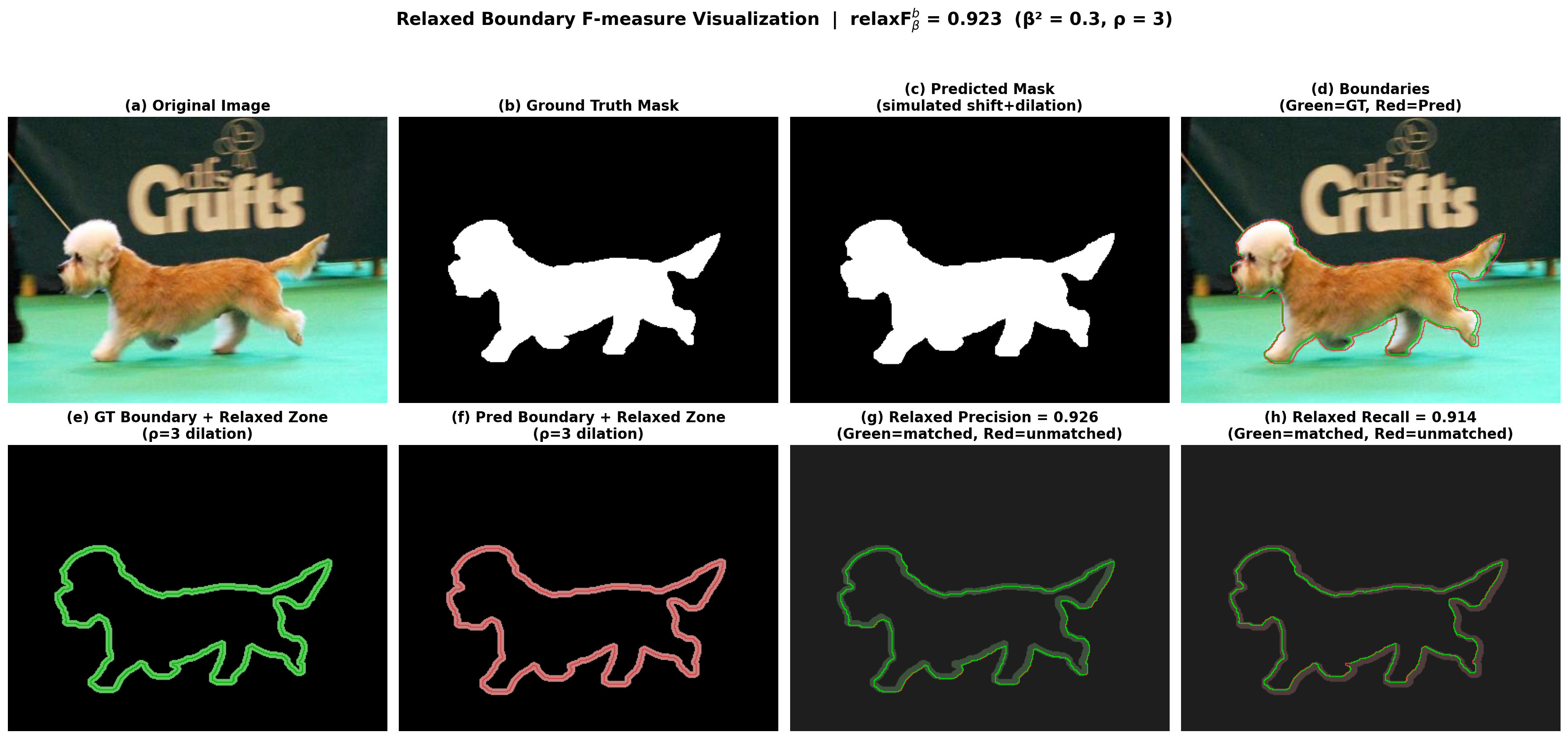
4. Relaxed Boundary F-measure

Standard evaluation metrics like region-based F-measure and MAE assess overall saliency map quality but are insensitive to boundary accuracy. A prediction that gets the interior right but has blurry edges can score well on these metrics while being visually unsatisfying. The relaxed boundary F-measure ($\text{relax}F_\beta^b$) directly evaluates how well predicted boundaries align with ground truth boundaries.

Step 1: Extract Boundaries

Given a saliency map $S$, first binarize it at threshold 0.5 to get $S_{bw}$. The boundary is extracted as a 1-pixel-wide contour using morphological operations:

\[\text{Boundary}(S_{bw}) = \text{XOR}(S_{bw},\ \text{Erode}(S_{bw}))\]

The XOR between the mask and its erosion leaves only the outermost pixel ring – the contour. The same operation extracts the ground truth boundary from $G$.

Step 2: Dilate Boundaries by $\rho$

A strict pixel-exact boundary match would be overly harsh – even a 1-pixel misalignment due to annotation ambiguity would count as an error. The relaxed metric introduces a slack parameter $\rho$ that allows boundary pixels to match within a tolerance band.

Each boundary is dilated by $\rho$ pixels (using a disk-shaped structuring element) to create a relaxed zone. In BASNet’s experiments, $\rho = 3$.

Step 3: Compute Relaxed Precision and Recall

Relaxed boundary precision ($\text{relax}\text{Precision}^b$) measures what fraction of predicted boundary pixels fall within $\rho$ pixels of any ground truth boundary pixel:

\[\text{relax}\text{Precision}^b = \frac{|\text{Pred boundary} \cap \text{GT relaxed zone}|}{|\text{Pred boundary}|}\]

Relaxed boundary recall ($\text{relax}\text{Recall}^b$) measures the reverse – what fraction of ground truth boundary pixels are within $\rho$ pixels of any predicted boundary pixel:

\[\text{relax}\text{Recall}^b = \frac{|\text{GT boundary} \cap \text{Pred relaxed zone}|}{|\text{GT boundary}|}\]

Step 4: Compute the F-measure

The relaxed boundary F-measure combines precision and recall using the standard $F_\beta$ formula:

\[\text{relax}F_\beta^b = \frac{(1 + \beta^2) \times \text{relax}\text{Precision}^b \times \text{relax}\text{Recall}^b}{\beta^2 \times \text{relax}\text{Precision}^b + \text{relax}\text{Recall}^b}\]

• $\beta^2 = 0.3$: weights precision more than recall (following convention in saliency evaluation)
• $\rho = 3$: the boundary slack in pixels

Visualizing Relaxed Boundary Matching

The following visualization uses a real image-mask pair from the DUTS-TE dataset. The “predicted” mask is simulated by slightly dilating and shifting the ground truth to create realistic boundary errors.

The 8-panel overview shows the full pipeline: from original image and masks, through boundary extraction, to the relaxed zones and precision/recall matching (green = matched within $\rho$, red = unmatched):

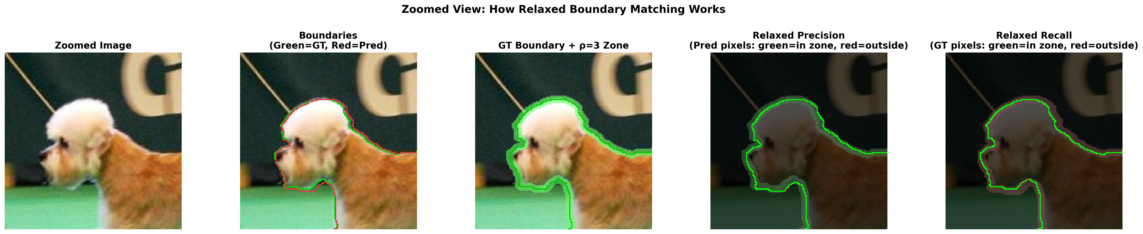
A zoomed view on the dog’s head region reveals the boundary matching at pixel level – showing exactly which predicted boundary pixels fall inside the GT relaxed zone and which fall outside:

Effect of the Slack Parameter $\rho$

The choice of $\rho$ directly controls how strict the boundary evaluation is. The visualization below shows the same prediction evaluated at four different slack levels:

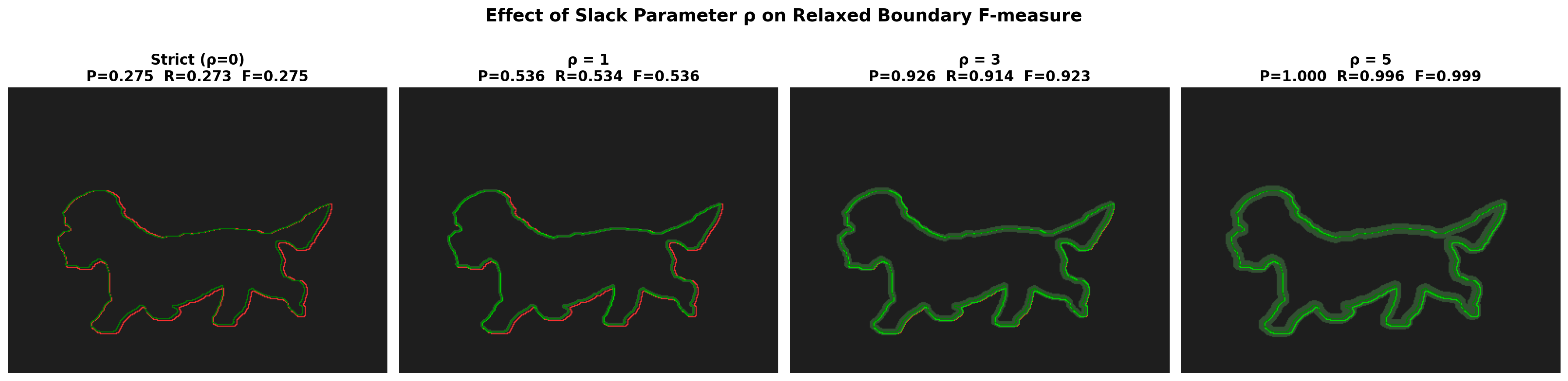
$\rho$	Precision	Recall	$F_\beta^b$	Interpretation
0 (strict)	0.275	0.273	0.275	Pixel-exact matching: very few boundary pixels align perfectly
1	0.536	0.534	0.536	1-pixel tolerance: captures ~half of near-boundary matches
3 (BASNet)	0.926	0.914	0.923	3-pixel tolerance: matches most boundary pixels despite slight shift
5	1.000	0.996	0.999	5-pixel tolerance: nearly all pixels match within this generous band

At $\rho = 0$, even a well-aligned prediction scores poorly because pixel-exact boundary matching is unrealistically strict. At $\rho = 3$, the metric captures genuine boundary quality while tolerating annotation ambiguity and minor sub-pixel misalignments. BASNet reports this metric across six benchmark datasets, demonstrating that its hybrid loss produces significantly better boundary quality than competing methods – improving $\text{relax}F_\beta^b$ by 4-6% over prior state-of-the-art.

---

Summary

U²-Net introduces the nested U-structure concept: replacing plain convolutional blocks with RSU blocks that are themselves miniature U-Nets. This captures multi-scale context at every encoder-decoder stage, enabling a 44M-parameter model trained from scratch to match methods using heavy pretrained backbones. The lightweight U²-Net† achieves competitive results at just 4.7 MB – 37x smaller.

BASNet contributes two complementary innovations. The hybrid loss ($\ell_{bce} + \ell_{ssim} + \ell_{iou}$) supervises at pixel, patch, and map levels, implicitly driving the network to produce sharp boundaries without explicit boundary annotations. The relaxed boundary F-measure provides a principled evaluation metric that captures boundary quality – filling a gap left by standard region-based metrics.

These ideas are independent and composable: U²-Net’s architecture can be trained with BASNet’s hybrid loss, and the relaxed boundary F-measure can evaluate any saliency method regardless of its architecture or training procedure.

---

Key References

Year	Paper	Contribution
2015	Ronneberger et al. — U-Net	The foundational encoder-decoder with skip connections
2019	Qin et al. — BASNet (CVPR)	Hybrid loss (BCE+SSIM+IoU) and relaxed boundary F-measure for boundary-aware saliency
2020	Qin et al. — U²-Net (Pattern Recognition)	Nested U-structure with RSU blocks; trains from scratch without pretrained backbone
2005	Ehrig & Euzenat — Relaxed Precision and Recall	Original formulation of relaxed matching (cited by BASNet as [7]); concept adapted for boundary pixel evaluation
2004	Wang et al. — SSIM (IEEE TIP)	Structural Similarity Index for perceptual image quality, repurposed as a training loss by BASNet