Video VLMs as Judges on Waymo's E2E Driving Set: A First-Principles Walkthrough

April 27, 2026

Target audience: ML practitioners with general transformer/VLM background who want to know whether off-the-shelf video vision-language models can sit in front of a human-rater queue on autonomous-vehicle scenario data — and what predictive uncertainty buys you in that role.

Why this question matters
The data: Waymo Open Dataset E2E challenge
Stitching 8 cameras into one VLM input
The judge setup — three video VLMs, one prompt
The TU / AU / EU framework — what each one measures
Analysis 1: greedy accuracy and variation under sampling
Analysis 2: per-clip predictive entropy from single-pass logits
Analysis 3: a real AU / EU split via prompt-paraphrase perturbation
The triage funnel — VLM as a router for human raters
What we still can’t measure
Key references

1. Why this question matters

Autonomous-vehicle perception teams generate driving log data faster than human annotators can label it. The standard pipeline looks like raw clip → human rater → training set, and the human is the bottleneck. A natural question: can a pretrained video VLM look at the clip first and decide what kind of scenario it shows — at minimum well enough to route clips to the right rater queue, or to flag the unusual ones for closer review?

This post walks through a small empirical study answering that question on Waymo’s End-to-End driving val set. We test three off-the-shelf video VLMs as zero-shot scenario classifiers, then ask not just are they accurate but do their confidence signals tell us anything useful. The headline finding is that only one of the three is calibrated well enough to be used as a triage signal, and getting to that conclusion requires distinguishing several different notions of “uncertainty” — which the post unpacks from first principles.

2. The data: Waymo Open Dataset E2E challenge

Waymo’s End-to-End driving dataset (WOD-E2E) is the camera-only benchmark from the 2024 challenge. Each sequence is 8 seconds of synchronized 8-camera video at 10 Hz, with ego pose and a small set of derived labels.

The label we care about for this experiment is the scenario cluster — a sequence-level tag drawn from a 10-class taxonomy that Waymo published with the challenge:

Cluster	What it captures
Intersections (manifest typo: `Interections`)	ego approaches / traverses an intersection — original typo preserved everywhere downstream so labels match the published manifest
Foreign Object Debris	something on the road that shouldn’t be there
Cyclist	a cyclist is the safety-relevant agent
Pedestrian	a pedestrian is the safety-relevant agent
Multi-Lane Maneuvers	ego changes between two or more lanes
Single-Lane Maneuvers	within-lane behavior (slowing, stopping, smooth following)
Special Vehicles	emergency vehicle, school bus, etc.
Cut_ins	another vehicle cuts into ego’s lane
Construction	construction zone present
Others	catch-all

Two facts about these labels matter for what follows:

Sequence-level, not frame-level. A “Cyclist” label means somewhere in the 8 seconds, the cyclist is the safety-relevant agent. It does not mean the cyclist is visible in every frame.
Sensor-suite-level, not single-camera-level. A “Cyclist” label does not say which camera the cyclist is in. We verified empirically that cyclist sequences often have the cyclist visible only in the rear cameras (CAM_7 and CAM_8) for most of the clip, entering the front camera briefly when ego passes them. This becomes important in the next section.

We sampled 5 clips per cluster × 10 clusters = 50 stratified clips from the val set as our eval set.

3. Stitching 8 cameras into one VLM input

Most video VLMs accept a single video as input — not an arbitrary set of cameras. So we composite the 8 cameras into a single 2×4-tile video at 4 Hz, then hand that to the model:

8-camera composite layout showing four forward-facing tiles in row 1 (FRONT_LEFT, FRONT, FRONT_RIGHT, SIDE_LEFT) and four mixed tiles in row 2 (SIDE_RIGHT, CAM_6, CAM_7 rear, CAM_8 rear), with a dashed cyclist trajectory traced from CAM_7 to CAM_8 to FRONT and a small ego-vehicle marker in the center.

Front-only judging would systematically miss most of the trajectory: a cyclist often appears first in the rear cameras (overtaking from behind), then in the side cameras, and only briefly in the front camera at the moment ego passes — and on clips where ego never overtakes, the cyclist never reaches the front camera at all.

Below is one of those exact cases — a cyclist visible in CAM_7 / CAM_8 (bottom-right tiles) for most of the clip, only entering the front camera near the end:

For comparison, here are three other clusters, all rendered as the same 8-camera composite:

Intersections — ego approaches an intersection:

Cut_ins — another vehicle cuts into ego’s lane:

Foreign Object Debris — object on the road:

These are the exact MP4 files passed into the VLMs in the experiments below.

4. The judge setup — three video VLMs, one prompt

We test three off-the-shelf, open-weights video VLMs:

Judge	Backbone	Why we picked it
Cosmos-Reason 2-2B	Qwen3-VL	NVIDIA’s reasoning-focused video VLM — native video input, small enough to run quickly
Video-LLaVA-7B	LanguageBind / Vicuna	Established baseline for video-language tasks
Molmo2-8B	Allen AI multimodal stack	Strong recent benchmark on video QA / grounding

All three receive the same composite video and a prompt that lists the 10 clusters and asks for the dominant scenario. Ground truth is Waymo’s published cluster label.

Single-pass logit-extraction pipeline: composite 8-camera video flows into the VLM, the multi-choice prompt is appended, the model's logits at the answer position are restricted to the 10 letter-token IDs A-J, softmaxed into a 10-class distribution, then summarized as a per-clip predictive entropy H of p.

One methodology bug worth naming up front

The first version of our eval set printed the cluster name in the title bar of every frame (Cyclist | seq 0fff5ea6 | frame 5/32). Both Cosmos and Video-LLaVA were reading the answer off the input, producing artificially high accuracy (62% and 70% respectively). After re-rendering the eval set without the title-bar text and re-running, accuracy collapsed to 20% and 10% — the leak was doing all the work. The numbers reported below are all from the leak-free clean run; the leaked run is preserved as a forensic artifact.

We then audited the remaining label-correlated channels: filenames passed to the model are anonymized sequence hashes (no cluster string), frame counts and codec metadata are constant across clusters, no EXIF is embedded in the rendered MP4s, and no prior turn in the prompt history contains the cluster name. The title-bar text was the only label-correlated signal we found; nothing rules out a subtler leak (e.g. resolution or compression artifacts that correlate with rendering pipeline), but the obvious surfaces are clean.

This is the failure mode where the measurement instrument contaminates the measurement. The takeaway: when an off-the-shelf model gives suspiciously good zero-shot numbers on a domain it was not trained on, look for the leak first.

Before we look at how the judges do, we need to set up the language we’re going to use to talk about their confidence. The next section is the measurement framework; the three analyses after it apply it.

5. The TU / AU / EU framework — what each one measures

Start with one number: Shannon entropy

A probabilistic classifier outputs a distribution $p$ over $K$ classes. The single scalar that summarizes “how uncertain is this prediction?” is Shannon entropy, in bits:

\[H(p) = -\sum_{i=1}^{K} p_i \log_2 p_i\]

$K$: number of classes (10 here)
$p_i$: probability the classifier assigns to class $i$
$H(p) \in [0, \log_2 K]$ — zero when one class has all the mass, $\log_2 K$ when the distribution is uniform

For our 10-class taxonomy, $H(p)$ ranges from 0 bits (model is certain) to $\log_2 10 \approx 3.32$ bits (model is uniformly clueless).

Why one number is not enough

$H(p)$ tells us how much the model is hedging. It does not tell us why. Two qualitatively different things can both raise entropy:

(a) The input is genuinely ambiguous. What’s left after model uncertainty has been integrated out — in practice, the within-sample entropy averaged over our chosen variability source. A coin flip is irreducibly 1 bit of entropy — no amount of training shrinks it. This is aleatoric uncertainty (from the Latin alea, die / chance — the randomness lives in the data, conditional on the chosen model class).
(b) The model doesn’t know. It spreads mass because it lacks the knowledge to commit, even on an input that is objectively clear-cut. This is epistemic uncertainty (from the Greek epistēmē, knowledge — the uncertainty lives in the model and would shrink with more training data).

Worth flagging up front: this AU/EU split is not setup-independent. Following Hüllermeier & Waegeman (2021), the decomposition is conditional on the choice of model class and the source of variability used to probe it — there is no setup-independent “amount of aleatoric uncertainty” in the data itself.

These two cases demand different responses. High aleatoric uncertainty means more annotators won’t help — the scene really is ambiguous. High epistemic uncertainty means more training data of this type will help — the model is the bottleneck. A single $H(p)$ blends them and forces you to guess which one you’re looking at.

A worked example: 8 weather forecasters

Imagine 8 forecasters each predicting “will it rain tomorrow?” — a binary outcome ($K=2$). Each forecaster outputs a distribution $p_i = [P(\text{rain}), P(\text{no rain})]$. We average them to get $\bar{p}$, then look at the three uncertainty numbers in three scenarios:

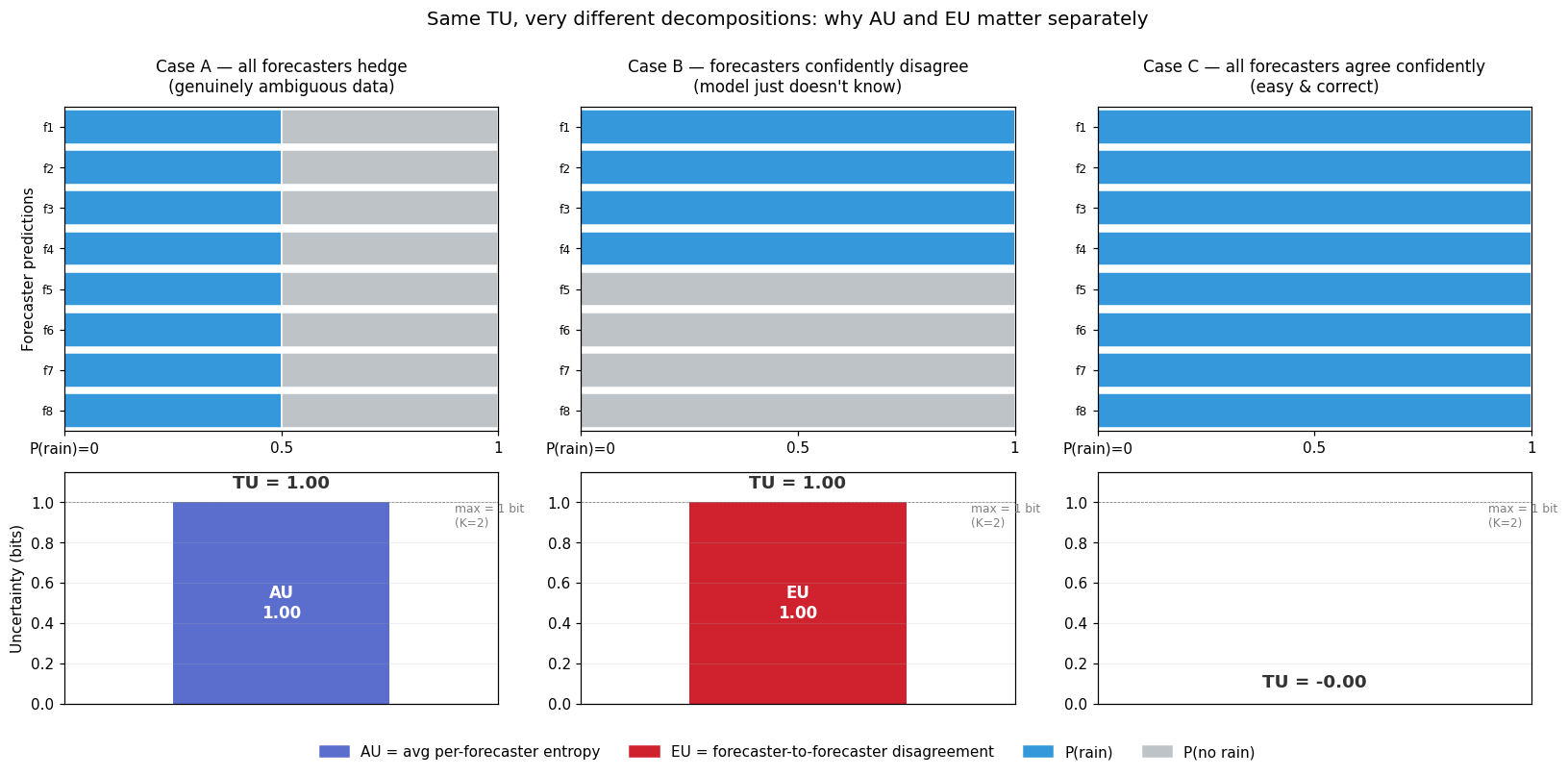
Scenario	Each forecaster says	$\bar{p}$	TU	AU	EU
A — genuinely ambiguous, forecasters agree	“[0.5, 0.5]” — coin flip, all 8 of them	[0.5, 0.5]	1.00	1.00	0.00
B — clear-cut data, forecasters disagree	4 say “[1, 0]”, 4 say “[0, 1]”	[0.5, 0.5]	1.00	0.00	1.00
C — clear-cut data, forecasters agree	all 8 say “[1, 0]”	[1, 0]	0.00	0.00	0.00

The key observation: Cases A and B have identical TU (1 bit, the maximum for $K=2$) but opposite operational meanings.

In Case A, the data really is a coin flip. Every forecaster individually hedges, all the spread lives within each forecaster’s own distribution, so AU = TU. Hiring more forecasters won’t help — there’s nothing to learn. Aleatoric.
In Case B, the data is clear-cut (some confident answer is right), but the forecasters confidently disagree. The spread doesn’t come from any individual hedging — it comes from disagreement across forecasters. Each $H(p_i)$ is zero, so AU = 0, and all the entropy lands in EU. Better-trained forecasters would converge on the right answer. Epistemic.

If you only saw $H(p) = 1$ bit, you couldn’t tell which case you were in — and you’d have no idea whether the right operational response was “hire a senior rater because the scene is ambiguous” or “collect more training data because the model is undertrained.” That is what the AU/EU split buys you.

Mapping back to the three VLM judges (Section 8 will show the actual numbers):

Cosmos is qualitatively in the Case A regime — on the AU-dominated side of the (AU, EU) plane — though with TU around 2 bits rather than the 1-bit ceiling of binary Case A, and AU at 2.07/3.32 ≈ 62% of the 10-class maximum. The model is hedged regardless of how you ask, but it is not maximally hedged.
Video-LLaVA sits at Case C for everything — low TU, AU and EU both near zero. The model is confident. (At 10% accuracy, that confidence is wrong, but that’s a calibration story, not an uncertainty-decomposition story.)
Case B (low AU + high EU = pure model disagreement) is empty in our data because prompt paraphrasing alone is not strong enough to make any of these models commit-then-disagree. Visual perturbation might populate it; we haven’t tested.

The trick to separating them: $N$ forward passes

With one distribution per clip, you can compute total entropy but you can’t decompose it. With $N$ stochastic forward passes per clip — each producing a full distribution $p_i$ — you get two questions you can answer separately:

“How spread is the average distribution $\bar{p} = \frac{1}{N}\sum_i p_i$?” That’s total uncertainty (TU). It captures both aleatoric and epistemic together.
“How spread is each individual distribution $p_i$, on average?” That’s the average per-trial entropy. Critically, this measures the minimum spread that any single trial already had. If even a perfect oracle would have given a spread distribution on this input, this term picks that up. So this is aleatoric uncertainty (AU).

What “stochastic forward pass” means is a design choice, and the choice determines what the resulting EU actually captures:

MC dropout / weight ensembles approximate posterior variability over model parameters — the canonical Bayesian-NN view of EU.
Temperature sampling at the output head probes decoding-noise variability, conditional on a fixed forward pass.
Prompt paraphrase probes language-side input sensitivity.
Temporal frame subsampling / camera dropout probes visual-side input sensitivity.

Strictly, classical EU is posterior uncertainty over model parameters — what BALD (Houlsby et al. 2011) formalizes as the mutual information $I(Y; \theta \mid x)$ between the prediction and the parameters. The input-perturbation route used here (prompt paraphrase, in Analysis 3) is a proxy for that, not the canonical setup; it conflates parameter uncertainty with input-sensitivity. We use it because it’s tractable on frozen black-box VLMs where we have no access to weights, and we are explicit about what it does and doesn’t measure.

The leftover — $\text{EU} = \text{TU} - \text{AU}$ — is the extra spread that came from trials disagreeing with each other. If every trial individually was confident but they confidently disagreed, AU is small but TU is large; the gap is model self-disagreement. Following Houlsby et al. (2011), this leftover equals the mutual information between the prediction and the variability source, which is the standard formulation of epistemic uncertainty.

The decomposition

\[\underbrace{H(\bar{p})}_{\text{TU}} \;=\; \underbrace{\frac{1}{N}\sum_{i=1}^{N} H(p_i)}_{\text{AU}} \;+\; \underbrace{H(\bar{p}) \;-\; \frac{1}{N}\sum_{i=1}^{N} H(p_i)}_{\text{EU}}\]

$N$: number of stochastic forward passes — the chosen variability source determines what the resulting EU captures (see the list above)
$p_i$: the model’s predictive distribution on trial $i$ (a 10-dim probability vector here)
$\bar{p} = \frac{1}{N}\sum_{i=1}^{N} p_i$: the mean predictive distribution across the $N$ trials
$H(p_i)$: Shannon entropy of one trial’s distribution, defined as in the first equation
TU $= H(\bar{p})$: how spread the averaged distribution is — total uncertainty
AU $= \frac{1}{N}\sum_i H(p_i)$: average per-trial entropy — uncertainty intrinsic to the input
EU $= \text{TU} - \text{AU}$: mutual information between prediction and trial-to-trial variability — model self-disagreement

Reading the (AU, EU) plane

The four corners of the plane have plain-words operational meanings:

Low AU + Low EU. Model is consistent and individually confident. Trustworthy.
High AU + Low EU. Model consistently says “this scene is ambiguous.” The data really is hard; defer to consensus.
Low AU + High EU. Model is confident on each pass but they disagree. Model doesn’t know — collect more training data.
High AU + High EU. Uncertain about everything. Escalate.

A single $H(p)$ number cannot distinguish these four cases — they all just look “high” or “low.” That is why we need the decomposition before we can talk about routing rules.

Setup-dependence caveat

The decomposition only works when each $p_i$ is a full distribution. If the trial-to-trial variability comes from sample-and-count (each trial returns one sampled class, i.e. a one-hot distribution), then $H(p_i) = 0$ for every trial, AU is forced to zero, and the decomposition collapses to $\text{EU} = \text{TU}$. This forces the design choice in Analysis 3, which uses prompt-paraphrase perturbation specifically to keep each $p_i$ a full softmax.

6. Analysis 1: greedy accuracy and variation under sampling

Greedy top-1 (one forward pass per clip, deterministic)

Judge	Top-1 vs Waymo	Distinct cluster strings predicted	Failure mode
Cosmos-Reason 2-2B	20% (10/50)	12 (case/spacing variants)	Defaults to `single_lane_maneuvers` on uncertain inputs
Video-LLaVA-7B	10% (5/50)	1 — `Intersections` × 50	Constant function — copies the prompt’s example values
Molmo2-8B	14% (7/50)	3 — Intersections (32), Multi-Lane (17), Cyclist (1)	Binary default; ignores 7 of 10 categories

Random baseline for 10-class classification is 10%. Cosmos is barely above chance, Video-LLaVA is chance, Molmo collapses to a coarser binary than the taxonomy expects. None of these models is usable as a labeling oracle on this dataset zero-shot.

But the more interesting observation is that all three fail differently. Cosmos hallucinates scene reasoning, VL ignores the video and copies the prompt, Molmo bins everything into two classes. Three failures with no shared signal is qualitatively different from “three judges making correlated errors,” and it shapes what the rest of the pipeline can do (more on this in Section 9).

Variation across 10 runs at temperature 0.3

Greedy decoding gives one answer per clip. To see how much each judge wobbles when allowed to sample, we re-ran the same 50 clips with temperature=0.3, do_sample=True, N=10 trials per clip, and looked at how often the 10 answers agreed:

Judge	Clips where all 10 trials agree (unanimous)	Most-common modal-vote prediction
Cosmos-Reason 2-2B	31 / 50	matches greedy answer on those 31 clips
Molmo2-8B	31 / 50	matches greedy answer on those 31 clips
Video-LLaVA-7B	8 / 50	wobbles substantially on the other 42

Cosmos and Molmo are deterministic-by-default even under sampling: on roughly two-thirds of clips they say the same thing 10 times in a row. Video-LLaVA is the opposite — it is the most variable judge under sampling, despite being the model that produced a perfectly constant Intersections answer under greedy decoding. Sampling exposes that VL has substantial probability mass on alternative tokens that greedy decoding hides; the constant-function behavior is an argmax artifact, not a narrow underlying distribution.

This sampling proxy is sparse — binary “did it flip-flop or not” for most clips — and it cannot tell the model is genuinely uncertain about a hard scene from the model is undertrained and randomly guessing. The next section produces a denser, continuous signal.

7. Analysis 2: per-clip predictive entropy from single-pass logits

There are two ways to get the $N$ stochastic predictions the AU/EU decomposition needs. The first — sample-and-count — runs $N$ forward passes with temperature > 0 and takes the sampled token from each. The second — single-pass logits — runs one forward pass with greedy decoding and reads the model’s full softmax distribution at the answer position.

Side-by-side comparison: sample-and-count (left, blue) shows 10 one-hot trial bars stacked vertically with their aggregate vote distribution and the formulas TU = H of p-bar, AU = expectation of H of p_i = 0 highlighted in red, EU = TU; single-pass logits (right, green) shows one continuous 10-class softmax distribution and the formula H(p) per clip.

The two approaches are not interchangeable for the AU/EU split:

In sample-and-count, each trial produces one sampled class. As a distribution that single answer is one-hot — [0, 0, 1, 0, ..., 0] — and the entropy of any one-hot is zero. So $\mathbb{E}_i!\left[H(p_i)\right] = 0$, $\text{AU} = 0$, $\text{EU} = \text{TU}$. We can measure TU but the decomposition collapses (this is the setup-dependence caveat from Section 5).
In single-pass logits, we get the model’s actual softmax distribution at the answer position from one forward pass. This is one full $p$ per clip — no $N$, no average. We can compute $H(p)$ directly as the per-clip predictive entropy, a continuous real-valued signal.

Neither method on its own produces a real AU/EU split. (For that you need $N$ forward passes and full per-trial distributions — Analysis 3 below does exactly that.) For this section we ran the single-pass logit version because it is roughly 16× cheaper in GPU time and the per-clip $H(p)$ it produces is denser and more usable than the sparse vote-distribution TU from $N=10$ sampling.

How we extracted the logits

out = model.generate(
    **inputs, max_new_tokens=1,
    output_scores=True, return_dict_in_generate=True,
    do_sample=False,                          # greedy
)
logits   = out.scores[0][0]                   # full vocab logits at answer position
class_logits = logits[letter_token_ids]       # restrict to A..J (the 10 cluster letters)
p        = torch.softmax(class_logits.float(), dim=0).cpu().numpy()
H        = -(p * np.log2(p + 1e-12)).sum()    # bits, ∈ [0, log2(10) ≈ 3.32]

The prompt is reformulated as multi-choice (each cluster gets a letter A-J, the model is asked to answer with one letter) so that the answer position is a single token. We restrict the vocab-sized logit vector to the 10 letter-token IDs and softmax to get a clean 10-class distribution.

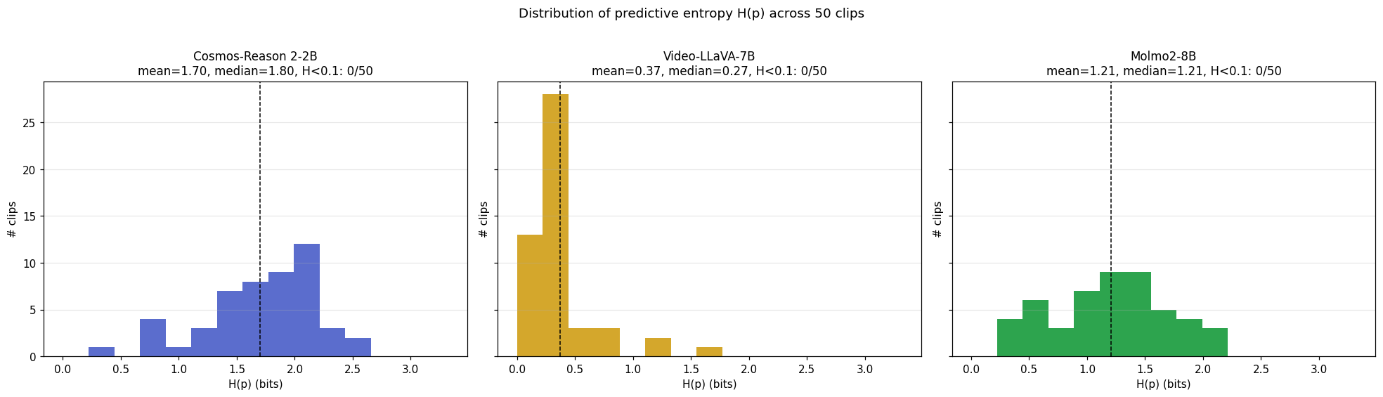
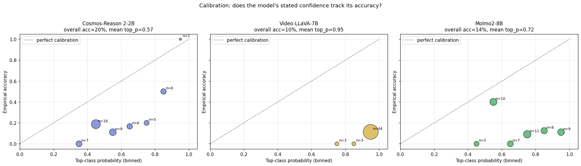
Headline numbers (50 clips × 3 judges, single-pass)

Judge	Top-1 acc	Mean $H(p)$	Mean top-class prob	$H(p)$ on correct	$H(p)$ on wrong	Escalation $\Delta$
Cosmos-Reason 2-2B	20%	1.700 bits	0.566	1.437	1.765	+0.329 ✓ informative
Video-LLaVA-7B	10%	0.374 bits	0.949	0.349	0.377	+0.027 ≈ noise
Molmo2-8B	14%	1.208 bits	0.718	1.352	1.185	−0.167 ✗ anti-informative

The escalation signal $\Delta$ is mean H(p) on wrong predictions − mean H(p) on correct predictions. If positive, the model is more uncertain when wrong — useful as a “flag for human review” signal. If negative, the model is more confident when wrong — actively misleading as a confidence proxy.

Per-cluster and distributional view

Grouped bar chart showing mean H(p) per cluster for each of the three judges across all 10 Waymo clusters, with a dashed reference line at the maximum entropy log2 of 10 ≈ 3.32 bits. Cosmos and Molmo bars are noticeably taller across most clusters than Video-LLaVA, which sits near zero on most.

Three-panel histogram showing H(p) split by correct (green) versus wrong (red) predictions for each judge. Cosmos shows wrong predictions clustering at higher entropy than correct ones (delta = +0.33 bits). Video-LLaVA shows almost all clips at low entropy regardless of correctness. Molmo shows correct predictions at higher entropy than wrong ones (delta = -0.17).

Three-panel histogram of the per-judge H(p) distribution across all 50 clips. Cosmos has a broad distribution centered around 1.7 bits, Video-LLaVA is sharply concentrated near zero, Molmo is roughly uniformly spread between 0.5 and 2.0 bits.

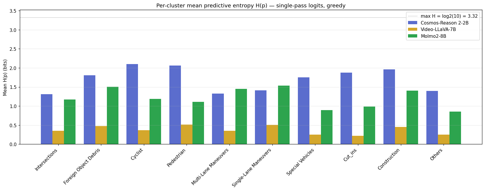
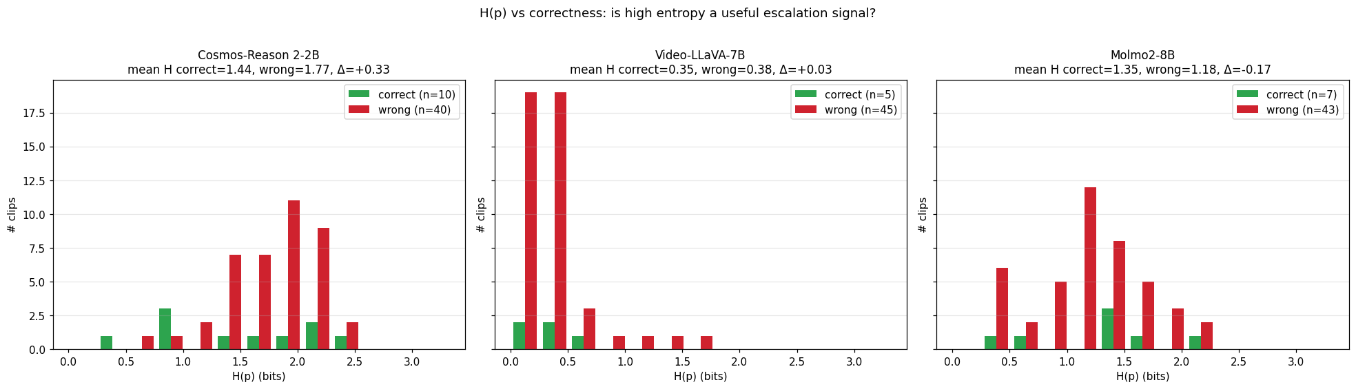
Cosmos’s H(p) is a continuous escalation signal

The +0.329 bit gap between wrong and correct predictions is in the right direction — wrong predictions sit on a wider distribution than correct ones (middle panel above). With only 50 clips (~10 correct, ~40 wrong for Cosmos) we don’t have the power to put a tight CI on $\Delta$; a bootstrap is the right next step and we haven’t run it. The gap is directionally consistent with the per-cluster picture below, but treat the magnitude as suggestive, not significant. The $H(p)$ from single-pass logits is continuous: every clip gets a real-valued entropy, so production code can do if H > 1.6: send to human rather than the binary did_it_flip_flop_under_sampling you would get from a vote-distribution proxy. A Cosmos-based learned evaluator can use $H(p)$ as a graded confidence score that orders clips by risk.

Video-LLaVA is severely overconfident

Mean top-class probability is 0.95 with top-1 accuracy of 10%. The reliability diagram makes this concrete — VL’s predictions live almost entirely in the 0.9-1.0 confidence bin, where empirical accuracy is ~10%. Any downstream pipeline that gated on top-class probability would over-trust this judge by an order of magnitude. The escalation signal $\Delta = +0.027$ is indistinguishable from noise — VL’s wrong and correct predictions are equally low-entropy.

Molmo’s H(p) goes the wrong way

Mean $H(p)$ on correct clips (1.35) is higher than on wrong clips (1.19). Two readings, both bad for production: either the correct answers happen on hard clips where Molmo is correctly uncertain (and lucky on the argmax), or the multi-choice letter-mapping interacts with Molmo’s tokenizer in a way that distorts the softmax. Either way, Molmo’s $H(p)$ cannot be used as an escalation signal — gating on H > threshold would systematically suppress correct answers.

Per-judge calibration must be measured, not assumed. Three judges, three different relationships between predicted confidence and empirical accuracy. A learned-eval framework that batched these 3 models behind a generic “if confidence high, accept” rule would silently produce a bias-amplifying pipeline.

8. Analysis 3: a real AU / EU split via prompt-paraphrase perturbation

Section 7 produced one full softmax per clip — enough for $H(p)$, not enough for AU / EU (which needs $N$ distributions). To get a real split we need multiple full distributions per clip — same model, same letter-mapping, different something. Two options: perturb the visual input ($N$ different temporal samplings, or $N$ camera-subsets) or perturb the language input ($N$ paraphrases of the question). We picked prompt paraphrasing because it is uniform across all 3 judges, requires zero video work, and is honestly scoped — it measures language-side sensitivity. Visual-side perturbation is a follow-up.

Setup

For each clip × judge × N=8 prompt phrasings (each a different framing of the same multi-choice question, with the same A-J letter→cluster mapping appended verbatim), we run one greedy forward pass and capture the full 10-class softmax. We then compute the decomposition from Section 5 on that list of 8 distributions.

Verification gate

Before applying to real data, the decomposition function (decompose(p_list) in analysis/uncertainty.py) is gated by 9 new tests added to the existing 21-test suite — covering unanimous one-hots ($\text{TU} = \text{AU} = \text{EU} = 0$), consistent uniform ($\text{TU} = \text{AU} = \log_2 K$, $\text{EU} = 0$ — pure aleatoric), disagreeing one-hots ($\text{AU} = 0$, $\text{EU} = \text{TU}$ — pure epistemic), the identity $\text{TU} = \text{AU} + \text{EU}$ on random Dirichlet samples, and Jensen’s inequality $\text{AU} \le \text{TU}$. All 30 tests pass before this section’s numbers exist.

On real data: identity holds to within $10^{-9}$ for all 50 × 3 = 150 decompositions, and AU is strictly positive on all 150 clips (sanity-checks that paraphrasing produced meaningful per-trial variation).

Headline numbers (50 clips × 3 judges, N=8 paraphrases per clip)

Judge	Modal acc	Mean TU	Mean AU	Mean EU	AU escalation $\Delta$	EU escalation $\Delta$
Cosmos-Reason 2-2B	22%	2.152 bits	2.065	0.087	+0.243	+0.011
Video-LLaVA-7B	10%	0.410 bits	0.391	0.019	+0.045	+0.004
Molmo2-8B	12%	1.591 bits	1.449	0.141	+0.111	−0.030

Two facts shape the rest of the section:

AU dominates EU by roughly 10× for all three judges. Almost all of the per-clip uncertainty under prompt paraphrasing is the model spreading mass within each phrasing’s distribution, not phrasings disagreeing with each other.
Cosmos’s AU is huge — 2.07 bits, 62% of the maximum possible entropy $\log_2 10 = 3.32$. The model is genuinely hedging on each individual answer.

The first fact is most visible as a stacked bar — bar height is total uncertainty TU, the blue base is AU, the red sliver on top is EU:

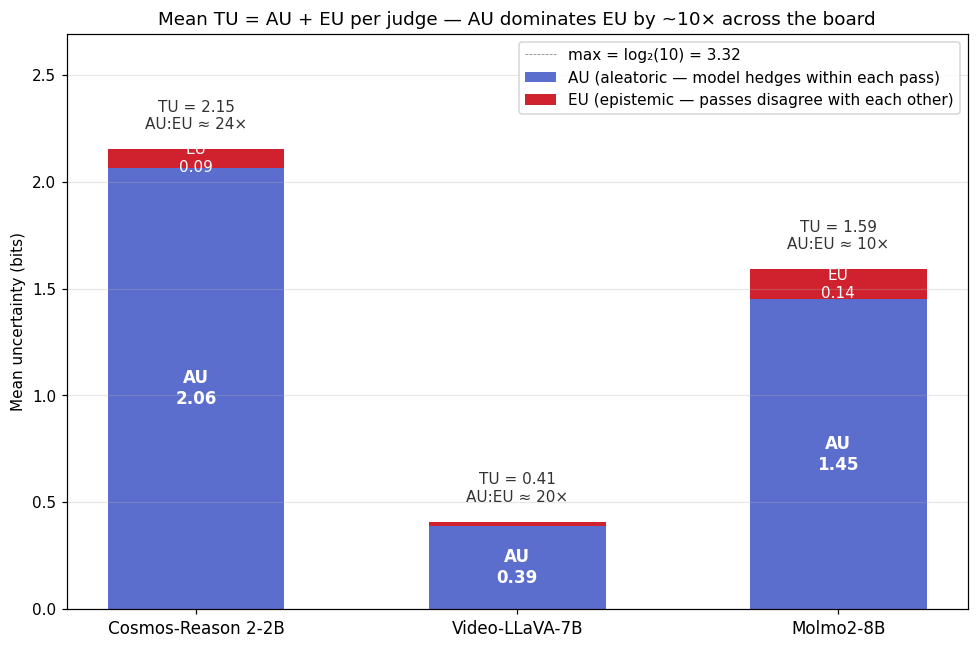
Stacked bar chart showing mean TU = AU + EU per judge. Cosmos's bar is tallest at 2.15 bits with AU=2.07 (blue) plus a small EU=0.09 sliver (red) on top, ratio AU:EU ≈ 24×. Molmo's bar is 1.59 bits with AU=1.45 plus EU=0.14, ratio ≈ 10×. Video-LLaVA's bar is shortest at 0.41 bits with AU=0.39 plus EU=0.02, ratio ≈ 21×. A dashed reference line at log₂(10)=3.32 marks maximum possible entropy.

In every bar, the red EU sliver is barely visible compared to the blue AU base. Whatever uncertainty these judges have under paraphrasing is uncertainty within each individual answer’s distribution, not disagreement across paraphrased answers. That tells us something specific: prompt paraphrasing isn’t a strong enough perturbation to shake any of these models loose from a stable predictive distribution. To populate the EU axis we’d need a perturbation that changes what the model sees (visual-side) — see “What this round explicitly doesn’t measure” below.

What this means: the model is consistent, but consistently uncertain

Reading the (AU, EU) plane from Section 5 against these numbers:

Low EU = the model gives the same kind of distribution regardless of which phrasing you use. The mean across 8 phrasings doesn’t differ much from any single phrasing. Operationally: robust to prompt choice.
High AU = each individual phrasing’s distribution is itself spread across multiple classes. The model is hedging within every single forward pass. Operationally: the model thinks the scene supports multiple labels.

Putting those together: all 3 judges are consistent across phrasings (low EU), but Cosmos and Molmo are individually uncertain (high AU); Video-LLaVA is individually narrow (low AU) and consistently narrow across phrasings (low EU) — i.e., consistently confidently-wrong. This corroborates the Analysis 2 finding (VL was 95% confident at 10% accuracy) through a completely different lens: VL’s narrowness is not an argmax artifact, and it is not paraphrasing-sensitive — the model just locks in.

Per-cluster picture

The same AU-dominates-EU story holds when broken out per cluster — bar height is mean TU for that cluster, blue is AU, red is EU on top:

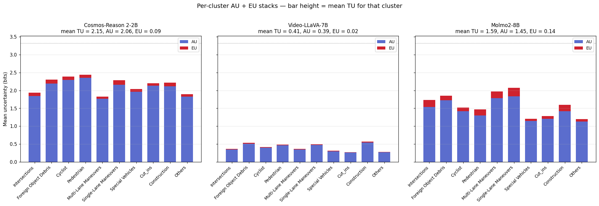
Three-panel stacked bar chart, one panel per judge, showing per-cluster mean TU = AU + EU. Cosmos's bars are uniformly tall (AU around 2 bits across nearly every cluster); EU slivers are tiny everywhere. Molmo's bars are moderate (AU around 1.5 bits); EU slivers slightly larger but still small. Video-LLaVA's bars are uniformly short (AU and EU both near zero across all clusters).

For Cosmos, mean AU is high across nearly every cluster — no easy/hard split, the model is broadly hedged. EU is a thin sliver everywhere. Same shape for Molmo at lower magnitude. VL is the odd one out — both AU and EU near zero on every cluster, which is the calibration story re-told.

The standalone per-metric breakdown (separate AU and EU panels) is also useful when you want to compare a single metric across judges directly:

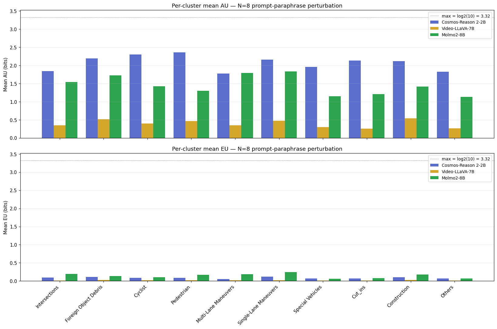
Two stacked grouped-bar charts. Top panel: per-cluster mean AU for the three judges across all 10 Waymo clusters; Cosmos's bars dominate, with Multi-Lane Maneuvers and Single-Lane Maneuvers near the maximum entropy ceiling. Bottom panel: per-cluster mean EU, with all three judges sitting near zero across the board.

AU vs EU per clip — the operational quadrant

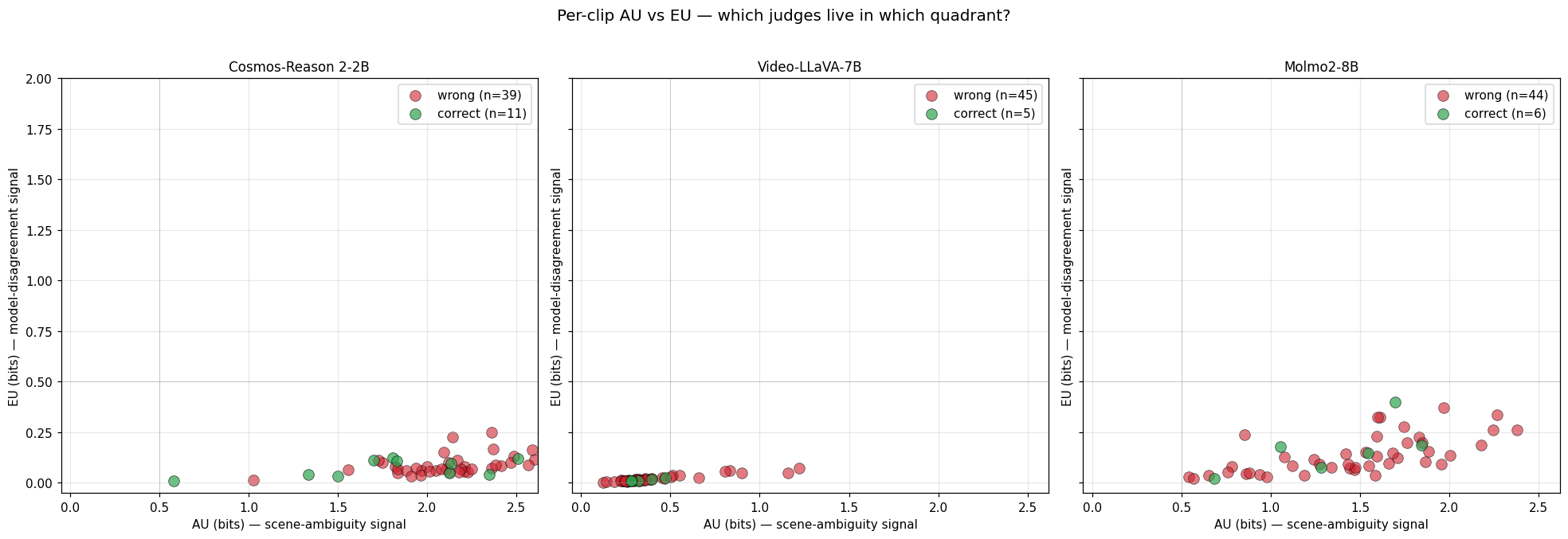
Empirically these three judges live in only two of the four (AU, EU) quadrants from Section 5:

Cosmos and Molmo: high AU, low EU — “the model is consistently saying ‘this scene is ambiguous to me’.” The dominant regime under prompt paraphrasing.
Video-LLaVA: low AU, low EU — “the model is consistently saying ‘I am sure’.” Combined with 10% accuracy, the worst possible calibration.
(High EU, low AU — “confident on each pass but they disagree” — is empty under prompt paraphrasing for these models. Visual perturbation would let us test whether that quadrant gets populated.)

AU and EU as escalation signals — which is the better wrong-answer flag?

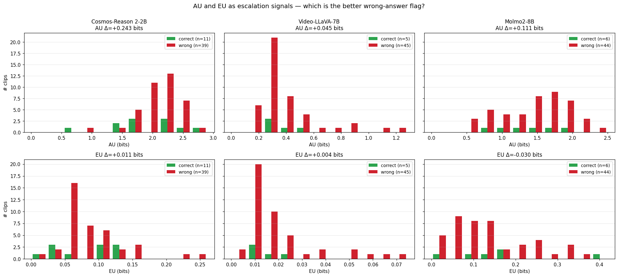
The AU row has signal — Cosmos’s wrong predictions sit on a wider distribution than correct ones (+0.243 bits, the strongest escalation Δ in this study). Molmo also shows a positive AU $\Delta$ (+0.111 bits), so Molmo’s AU is more usable as an escalation signal than its Analysis 2 $H(p)$ was (which went the wrong way at −0.167). The EU row is indistinguishable from noise for all three judges, which makes operational sense given the paraphrase-consistency finding. The same small-sample CI caveat from Analysis 2 applies to these Δ values — the per-cluster picture above is the more robust read.

What this round explicitly doesn’t measure

This round measures language-side uncertainty only. The follow-up is visual-side perturbation: re-render each clip with $N$ different temporal samplings (different 8-second windows of the same scene) or $N$ different camera dropouts (front-only, rear-only, side-only). That setup would let us test whether EU grows — the prediction would be expected to populate the high-EU quadrant if it is sensitive to which 8-second window or which cameras the model sees (e.g. the prediction may flip when the cyclist drops out of CAM_7+CAM_8) — and we could compare that EU against the AU we measured here. The clean version of the operational story is “AU from prompt paraphrasing + EU from visual perturbation”; this round only delivers half of that.

9. The triage funnel — VLM as a router for human raters

The point of this experiment is not to replace human raters with VLMs — none of the three judges is accurate enough for that, and the AV labeling problem is too high-stakes to hand to a 20%-accurate model. The point is to use the VLM as a router that splits the incoming clip stream into the right downstream queue:

Each branch maps to a different downstream cost: auto-bin is the cheapest (no human touch), standard human review is the baseline, and novel-scenario candidate is the most interesting — if the VLMs collectively give up and the class distribution looks like the model is groping, the clip might not fit any of the existing 10 categories, and routing it to a taxonomy-review queue lets the dataset evolve. From our 50-clip sample, 0 clips had all-3-agree-and-correct, which is a function of how bad these particular zero-shot judges are; a fine-tuned Cosmos would change this. The load-bearing artifact is the rule table at the end of this section — what follows is the gating logic that justifies it.

Per-judge gating, not per-pipeline gating

The calibration findings from Sections 7 and 8 are the gating constraint on this design. Only Cosmos’s $H(p)$ and AU are monotonic with correctness — Video-LLaVA’s confidence is meaningless (95% confident at 10% accuracy), and Molmo’s $H(p)$ goes the wrong way (its AU under paraphrasing partially recovers, but its single-pass $H(p)$ does not). So the practical funnel uses Cosmos’s signals as the primary uncertainty gate, with the other two judges contributing as cross-judge agreement checks rather than as confidence sources. Routing rules cannot be uniform across judges — they must be derived per judge from a calibration set.

AU as the primary signal, EU as a secondary check

The single-pass $H(p)$ from Analysis 2 was the original proposal for gating because it was the only signal that monotonically tracked correctness. Analysis 3 lets us do better: route by AU, with EU as a secondary “did the model give different confident answers under paraphrasing?” check that flags clips for prompt-robustness review specifically. The expanded routing rule:

Bucket	Trigger	Downstream
Auto-bin	low AU AND all 3 judges’ modal predictions agree	batch-accept the cluster label
Standard human review	high AU OR judges disagree	regular rater queue
Prompt-robustness review	high EU (rare under paraphrasing, common under visual perturbation when we add it)	prompt-design audit + senior rater
Novel-scenario candidate	high AU AND no judge confident AND $\bar{p}$ is roughly uniform	taxonomy-review queue

The funnel diagram still applies; Analysis 3 just splits the “high-uncertainty” branch into AU-driven and EU-driven sub-branches, giving the human rater more information about why the VLM is uncertain.

What happens inside the novel-scenario branch

Routing a clip to “taxonomy-review queue” only specifies where it goes — not what to do once it gets there. The follow-up post Discovering New Scenarios in Waymo’s ‘Others’ Bucket demonstrates the downstream pipeline: caption every flagged clip with two independent VLMs, embed and cluster each captioner’s outputs separately, and surface only the cluster pairs that survive a permutation-test cross-validation. Run on Waymo’s 22 Others-labeled val clips, exactly one cluster pair survives the gate (Jaccard 0.60, $p < 0.05$), and what the discovered cluster actually contains turns out to say more about how labelers handle ambiguous lighting than about a missing event category.

10. What we still can’t measure

Two known gaps remain:

Cross-judge ensemble calibration. Section 9’s design uses three judges as cross-checks, but we have not measured whether ensemble agreement (e.g. all-3-confidently-agree) is itself a calibrated signal. Probably not on this small sample — and given that all 3 judges fail differently, an ensemble may be no better calibrated than any single one. Worth running on a ≥500-clip set before deploying anything.

No fine-tuning baseline. All three judges are zero-shot. The natural comparison is Cosmos with LoRA fine-tuning on a 200-clip Waymo-labeled subset — based on similar literature, expect a 30-50 percentage-point lift on top-1 accuracy. The interesting question is whether fine-tuning also improves the calibration of $H(p)$ and AU, or whether the model just gets more confidently wrong.

11. Key references

Year	Paper / Resource	Relevance
2011	Houlsby et al., Bayesian Active Learning by Disagreement (BALD)	The mutual-information formulation of epistemic uncertainty used in the TU = AU + EU decomposition
2017	Kendall & Gal, What Uncertainties Do We Need in Bayesian Deep Learning?	Canonical reference for the aleatoric / epistemic split in deep models
2018	Depeweg et al., Decomposition of Uncertainty in Bayesian Deep Learning for Efficient and Risk-Sensitive Learning	The exact AU/EU decomposition we used
2024	Waymo, End-to-End Driving Dataset / Challenge	The dataset and the 10-cluster taxonomy
2024	LanguageBind / Lin et al., Video-LLaVA	One of the three judges
2024	NVIDIA, Cosmos-Reason 2	One of the three judges (Qwen3-VL-based)
2024	Allen AI, Molmo / Molmo2	One of the three judges
2017	Guo et al., On Calibration of Modern Neural Networks	Background on reliability diagrams and the kind of post-hoc recalibration (Platt scaling, isotonic) that would be the next step for any of these three judges before production use