Distilling a 6B Image Model with LADD: Architecture, Experiments & Hard Lessons
April 5, 2026
Target audience: ML engineers familiar with diffusion models who want to understand how adversarial distillation works in practice — including the parts that break.
This is Part 2 of our series on distilling Z-Image, a 6.15B parameter text-to-image model. Part 1 covered data curation — how we assembled 500K diverse prompts from 9 sources. This post covers the training framework: the architecture, the loss function, hyperparameter tuning, scaling to 8 GPUs with FSDP, and the blunders that taught us the most.
Table of Contents
- Overview
- Architecture & Code
- Experimental Setup
- Hyperparameter Search Results
- Training Metrics: What to Watch and What Breaks
- What We Observed
- Technical Difficulties
- Lessons Learned
- Summary & Next Steps
- Appendix: Anti-Mode-Collapse Sweep
- Key References
1. Overview
The goal is simple to state: take a 50-step diffusion model and make it generate images in 4 steps, with minimal quality loss. The method is LADD — Latent Adversarial Diffusion Distillation (Sauer et al., 2024).
Unlike traditional knowledge distillation that minimizes MSE between teacher and student outputs, LADD uses adversarial training — a GAN (Generative Adversarial Network) — in the teacher’s latent feature space. A lightweight discriminator learns to distinguish teacher features from student features, and the student learns to fool it. No pixel-space losses, no perceptual networks, no FID-optimizing tricks — just a GAN operating on frozen teacher representations.
The setup involves three models cooperating in a delicate balance:
| Component | Parameters | Role | Trainable |
|---|---|---|---|
| Student (S3-DiT) | 6.15B | Denoises in fewer steps | Yes |
| Teacher (S3-DiT) | 6.15B | Provides feature representations | No (frozen) |
| Discriminator (Conv heads) | 14M | Multi-scale adversarial feedback | Yes |
| Text Encoder (Qwen3) | ~3B | Encodes prompts | No (frozen) |
| VAE (AutoencoderKL) | ~0.5B | Latent ↔ pixel conversion | No (frozen) |
The student is initialized as an exact copy of the teacher. Training teaches it to skip steps — to produce in 4 steps what the teacher produces in 50.
2. Architecture & Code
This section covers the three core components — the LADD architecture, the discriminator design, and the loss function that ties them together.
2.1 The LADD Architecture

The architecture has three key ideas that separate it from simpler distillation approaches.
Idea 1: The student predicts velocity, not noise
Z-Image uses flow matching (Lipman et al., 2023) — a framework where, unlike noise-prediction diffusion (DDPM), the forward process interpolates linearly between data and noise, and the model predicts the velocity of that interpolation:
\[x_t = (1 - t) \cdot x_0 + t \cdot \varepsilon\]- $x_0$: clean latent (teacher-generated with CFG=5, 50 steps)
- $\varepsilon$: Gaussian noise
- $t$: timestep in $[0, 1]$ — higher means noisier
The student predicts a velocity $v_\theta$ and we recover the denoised latent:
\[\hat{x}_0 = x_t - t \cdot v_\theta(x_t, t, c)\]- $v_\theta$: student’s velocity prediction
- $c$: text conditioning from Qwen3
This is implemented in train_ladd.py:824:
# Convert velocity to denoised latent: x̂_0 = x_t - t * v
student_pred = x_t - t_bc * student_velocity
Idea 2: Re-noising creates a shared comparison space
The student’s denoised prediction $\hat{x}_0$ and the teacher’s clean latent $x_0$ can’t be compared directly by the discriminator — they might be at different quality levels for trivial reasons (the student just started training). Instead, both are re-noised to a shared noise level $\hat{t}$, sampled from a logit-normal distribution — a distribution that applies a sigmoid to a Gaussian sample, concentrating values in $(0, 1)$ away from the extremes:
\[\text{fake: } (1 - \hat{t}) \cdot \hat{x}_0 + \hat{t} \cdot \varepsilon_1\] \[\text{real: } (1 - \hat{t}) \cdot x_0 + \hat{t} \cdot \varepsilon_2\]This ensures the discriminator sees a smooth mix of noise levels rather than specializing on one scale.
From ladd_utils.py:59-76:
def logit_normal_sample(batch_size, m=1.0, s=1.0, device="cpu", generator=None):
    """Sample from logit-normal: u ~ Normal(m, s²), t = sigmoid(u)."""
    u = torch.normal(mean=m, std=s, size=(batch_size,), generator=generator, device=device)
    t = torch.sigmoid(u)
    t = t.clamp(0.001, 0.999)
    return t
Idea 3: Gradients flow through the frozen teacher
This is the subtlest part. The teacher’s weights are frozen (requires_grad_(False)), but on the fake path, the computation graph is kept alive — no torch.no_grad(). This means gradients flow backward through the teacher’s operations to reach the student:
student → x̂₀ → re-noise → teacher(forward, no_grad on weights) → disc → g_loss
                                    ↑ gradients flow through here
The real path uses torch.no_grad() because no gradient is needed — it’s just providing a reference.
From train_ladd.py:914-920:
# Teacher forward WITH gradient graph (frozen weights, live graph)
_, fake_extras_grad = teacher(
    fake_input_grad,
    t_hat,
    prompt_embeds,
    return_hidden_states=True,
)
2.2 The Discriminator Design

The discriminator is not a full model — it’s 6 independent lightweight heads, each attached to a different layer of the teacher transformer. This multi-scale design is what makes LADD work with only 14M parameters (0.2% of the student).
Why multiple layers?
Each teacher transformer block captures different abstractions:
| Layers | What they capture | Why it matters |
|---|---|---|
| 5, 10 | Texture, local patterns | Catches blurriness, color artifacts |
| 15, 20 | Object composition, spatial relationships | Catches structural errors |
| 25, 29 | Semantics, prompt alignment | Catches meaning drift |
If the discriminator only watched one layer, the student could learn to fool that specific abstraction level while degrading at others. Six layers make gaming the system much harder.
Head architecture
Each head is a small convolutional network with FiLM conditioning (Feature-wise Linear Modulation) from the timestep and text embedding. FiLM works by learning a per-channel scale and shift from the conditioning signal, so the discriminator can adjust which features matter depending on the noise level and prompt:
From ladd_discriminator.py:67-72:
cond = torch.cat([t_embed, text_embed], dim=-1)   # conditioning signal
film_params = self.cond_mlp(cond)                  # MLP predicts scale+shift
scale, shift = film_params.chunk(2, dim=-1)        # split in half along last dim
h = h * (1.0 + scale) + shift                     # modulate features
The MLP outputs a vector of size hidden_dim * 2 (512), and .chunk(2, dim=-1) splits it into two halves of 256 each — one for scale, one for shift. Each feature channel gets its own modulation: a scale near 0 suppresses that channel, a large scale amplifies it.
The full head architecture from ladd_discriminator.py:18-85:
class LADDDiscriminatorHead(nn.Module):
    def __init__(self, feature_dim=3840, hidden_dim=256, cond_dim=256):
        super().__init__()
        # FiLM conditioning: timestep + text → scale, shift
        self.cond_mlp = nn.Sequential(
            nn.Linear(cond_dim * 2, hidden_dim),
            nn.SiLU(),
            nn.Linear(hidden_dim, hidden_dim * 2),  # scale + shift
        )
        self.proj = nn.Linear(feature_dim, hidden_dim)

        # 2D conv layers (applied after reshaping tokens to spatial layout)
        self.conv1 = nn.Conv2d(hidden_dim, hidden_dim, 3, padding=1)
        self.gn1 = nn.GroupNorm(32, hidden_dim)
        self.conv2 = nn.Conv2d(hidden_dim, hidden_dim // 2, 3, padding=1)
        self.gn2 = nn.GroupNorm(16, hidden_dim // 2)
        self.conv_out = nn.Conv2d(hidden_dim // 2, 1, 1)
The pipeline per head: Linear projection (3840→256) → FiLM modulation (scale + shift from timestep and text) → reshape to 2D spatial → two conv blocks with GroupNorm → 1×1 conv → global mean pool → scalar logit.
All 6 head logits are summed into total_logit for the final real/fake decision:
for layer_idx in self.layer_indices:
    head_logits = self.heads[str(layer_idx)](img_feats, spatial_size, t_embed, text_embed)
    total_logit = total_logit + head_logits
2.3 Loss Function & Training Loop

The hinge loss
LADD uses the hinge loss variant of adversarial training — the same loss used in spectral normalization GANs. It has a nice property: the discriminator loss saturates once it’s confident, preventing it from becoming arbitrarily strong.
From ladd_discriminator.py:202-216:
@staticmethod
def compute_loss(real_logits, fake_logits):
    """Hinge loss for GAN training."""
    d_loss = torch.mean(F.relu(1.0 - real_logits)) + torch.mean(F.relu(1.0 + fake_logits))
    g_loss = -torch.mean(fake_logits)
    return d_loss, g_loss
Discriminator loss pushes real logits above +1 and fake logits below -1. Once confident, the ReLU clips to zero — no further gradient signal. This prevents the discriminator from running away.
Generator (student) loss is simply $-\mathbb{E}[\text{fake logits}]$ — maximize the discriminator’s score on student outputs.
The asymmetric update schedule
The discriminator and student don’t update at the same frequency. The discriminator updates every step, while the student updates only every $N$ steps (gen_update_interval):
From train_ladd.py:802, 887-944:
is_gen_step = (global_step % args.gen_update_interval == 0)

# Discriminator: always update
accelerator.backward(d_loss)
disc_optimizer.step()

# Student: update every N steps
if is_gen_step:
    accelerator.backward(g_loss_update)
    student_optimizer.step()
Why? The discriminator needs to stay ahead of the student to provide useful gradient signal. If both update every step, they oscillate. The discriminator uses a 10× higher learning rate (5e-5 vs 5e-6) for the same reason.
Timestep curriculum
The student sees a mix of denoising difficulties, with a curriculum that shifts from easy to hard:
From train_ladd.py:408-440:
student_timesteps = [1.0, 0.75, 0.5, 0.25]

if global_step < warmup_steps:
    # Warmup: only easy tasks (shown for n=4; source computes dynamically)
    probs = [0.0, 0.0, 0.5, 0.5]
else:
    # Main phase: heavily favor t=1.0 (full denoising — the hard case)
    probs = [0.7, 0.1, 0.1, 0.1]
At $t = 1.0$, the student starts from pure noise — this is the hardest case and what matters most for few-step inference. At $t = 0.25$, it starts from a mostly-clean input. The curriculum warms up on easy cases before emphasizing the hard one.
3. Experimental Setup
Our experimental pipeline had four stages: precompute, small-run sweeps, KID evaluation, and cluster launch.
3.1 Precomputing latents and embeddings
Training LADD requires teacher-generated latents (50-step generation with CFG=5) for every training prompt. We precomputed these offline along with Qwen text embeddings and CLIP embeddings for discriminator conditioning. This avoids the cost of running the teacher during training and allows the frozen teacher to focus solely on feature extraction.
We benchmarked precomputation throughput:
| Batch size | Time per image | Peak VRAM |
|---|---|---|
| 1 | 8.9s | 21.9 GB |
| 4 | 7.5s | 25.2 GB |
| 8 | 7.3s | 29.5 GB |
At 7.3s/image with embarrassingly parallel sharding (each GPU processes an independent subset of prompts, no communication needed), precomputing all 500K latents across 8 A100s would take:
\[\frac{500{,}000 \times 7.3}{8} = 456{,}250 \text{ seconds} \approx 127 \text{ hours}\]We had 6 hours of compute. The math was brutal: we could precompute roughly 10K latents in 4 hours — 2% of our dataset. Training would repeat each latent ~128 times over 20K steps. This was a hard trade-off we should have modeled before curating 500K prompts (more on this in Section 7).
3.2 Small runs on 3K subsets
For hyperparameter tuning, we took inspiration from Andrej Karpathy’s autoresearch concept — have an AI agent run experiments autonomously overnight. We built a lightweight framework around this idea:
research/experiment.py— the only file the agent modifies. Hyperparameters are constants at the top; the script generates a bash command, trains, evaluates, and logs to W&B.research/program.md— agent instructions: read prior results, propose the next experiment, modifyexperiment.py, run it, record the result, repeat.research/results.tsv— experiment log (commit hash, KID, VRAM, status, description).
Each experiment ran 500 steps on a single A100 80GB (the debug split: 98 prompts or 3K subset, 512px). The agent ran autonomously for ~8 hours overnight, completing 21 experiments across two rounds.
3.3 KID evaluation and config selection
We used KID (Kernel Inception Distance) — an unbiased metric preferred over FID for small sample sizes — to evaluate each run. Lower is better. The untrained student (teacher weights, zero LADD training) scores KID = 0.0689. We kept only configs that beat this baseline.
A critical finding: repeated runs of the exact same config show significant variance at 500 steps with bs=1:
| Run | KID |
|---|---|
| exp3 (original) | 0.0582 |
| run2 | 0.0692 |
| run3 | 0.0700 |
| run4 | 0.0658 |
| run5 | 0.0675 |
| Mean ± Std | 0.0661 ± 0.0044 |
The best single run (0.0582) was a lucky outlier — the true improvement is ~4% over the untrained baseline (0.0689), not 15.5%. This variance is inherent to bs=1 adversarial training over only 500 steps: each run sees the data in a different random order, and GPU non-determinism compounds.
Additionally, 1000 steps degrades on 3K data: 5-run mean KID = 0.0913 ± 0.0044 at 1000 steps vs 0.0661 ± 0.0044 at 500 steps. The student overfits — it memorizes the discriminator’s feedback on the small dataset rather than learning general features. More training data (10K+) is needed before longer training helps.
Lesson: Never trust a single run. Run at least 3-5 seeds and report the mean. A single lucky result can be 2× better than the true mean, leading to false confidence in a configuration. The variance also means that improvements below ~5% are within noise.
3.4 Cluster launch
Once we identified the best config from the small-run sweeps, we launched on the full 8-GPU cluster with 10K precomputed latents.
From training/train_ladd.sh:
accelerate launch \
    --config_file training/fsdp_config.yaml \
    training/train_ladd.py \
    --train_batch_size=4 \
    --gradient_accumulation_steps=2 \
    --max_train_steps=20000 \
    --learning_rate=5e-6 \
    --learning_rate_disc=5e-5 \
    --gen_update_interval=3 \
    --mixed_precision=bf16 \
    --gradient_checkpointing \
    --checkpointing_steps=2000 \
    --validation_steps=2000
Effective batch size: $4 \times 8 \times 2 = 64$. Target: 20K steps in ~2 hours.
3.5 What we tuned (and in what order)
LADD has several hyperparameters that interact in non-obvious ways. Here’s what each one controls:
| Hyperparameter | What it controls | Default | Why it matters |
|---|---|---|---|
student_lr |
Student optimizer learning rate | 5e-6 | Too high → divergence. Too low → slow learning. |
disc_lr |
Discriminator learning rate | 5e-5 | Must stay ahead of student (typically 10× higher). |
gen_update_interval (GI) |
Discriminator steps per student update | 5 | Controls D/G balance — the most sensitive knob. |
renoise_m |
Logit-normal mean for re-noising $\hat{t}$ | 1.0 | Controls what noise level the discriminator mostly sees. Higher → more noise → harder to distinguish. |
renoise_s |
Logit-normal std for re-noising $\hat{t}$ | 1.0 | Controls spread of noise levels. Wider → more diversity in discriminator feedback. |
disc_layer_indices |
Which teacher layers get discriminator heads | [5,10,15,20,25,29] | Determines which abstraction levels are supervised. |
disc_hidden_dim |
Hidden dimension per discriminator head | 256 | Controls head capacity — too large → overfitting, too small → underfitting. |
We tuned them in this order, each time fixing the best value and moving on:
- Learning rates (student_lr, disc_lr) — establish stable training dynamics first
- Generator update interval (GI) — the D/G balance knob with the most impact
- Noise schedule (renoise_m, renoise_s) — controls discriminator’s operating point
- Discriminator architecture (layer_indices, hidden_dim) — structural choices, tuned last
4. Hyperparameter Search Results
We ran three rounds of sweeps (33+ experiments total), each building on lessons from the previous round.
Round 1: Pre-fix sweep (broken pipeline)
These results used KID (Kernel Inception Distance). Lower is better.
Noise schedule exploration — tuning the logit-normal distribution parameters for re-noising:
renoise_m |
renoise_s |
KID | vs baseline |
|---|---|---|---|
| 1.0 (default) | 1.0 | 0.00804 | — |
| 0.0 | 1.0 | 0.00551 | -31% |
| 0.5 | 1.0 | 0.00461 | -43% |
| -0.5 | 1.0 | 0.00508 | -37% |
| 0.5 | 0.5 | 0.00564 | -30% |
| 0.5 | 1.5 | 0.00559 | -30% |
The default $m = 1.0$ was too high — sigmoid(1.0) ≈ 0.73, meaning the discriminator mostly saw high-noise samples where real and fake are hard to distinguish. $m = 0.5$ (sigmoid(0.5) ≈ 0.62) shifted the distribution toward moderate noise levels where the discriminator gets more useful signal.
Generator update interval — how many discriminator steps per student update:
| GI | KID | vs baseline |
|---|---|---|
| 2 | 0.01102 | +37% (worse) |
| 3 | 0.00804 | baseline |
| 4 | 0.00241 | -70% |
| 6 | 0.00202 | -75% |
| 8 | 0.00087 | -89% |
| 10 | 0.01290 | +60% (worse) |
GI=8 was a dramatic win — 89% better than baseline. But this turned out to be an artifact of the broken pipeline (see Section 8).
Discriminator architecture — we also tested head configurations:
| Config | KID | Notes |
|---|---|---|
| 6 layers [5,10,15,20,25,29], dim=256 | 0.000869 | best |
| 3 layers [10,20,29] | 0.001469 | 69% worse |
| 8 layers [3,7,11,15,19,23,27,29] | 0.001513 | 74% worse |
| dim=128 | 0.001184 | 36% worse |
| dim=512 | 0.006385 | 635% worse |
The original 6-layer, 256-dim config was already optimal. More layers added noise without new signal; larger hidden dims made the heads harder to train.
Full results tracked in research/results.tsv.
Round 2: Post-fix sweep (corrected pipeline)
After fixing 5 critical bugs, we re-ran the sweep. The results shifted significantly:
| Experiment | Config change | KID | vs baseline |
|---|---|---|---|
| baseline | slr=5e-6, dlr=5e-5, GI=8 | 0.0637 | — |
| exp1 | dlr=1e-5 (lower disc LR) | 0.0624 | -2% |
| exp2 | GI=3 (was 8) | 0.0589 | -7.5% |
| exp3 | slr=2e-5 (higher student LR) | 0.0792 | +24% (worse) |
| exp4 | GI=3 + dlr=1e-5 | 0.0616 | -3.3% |
The optimal GI flipped from 8 to 3 after fixing the pipeline. Why? In the broken pipeline, “real” samples were just noise-mixed-with-noise — trivially easy for the discriminator. It needed many steps to avoid overwhelming the student. With proper teacher latents as real samples, the discrimination task became genuinely hard, and the student needed more frequent updates to keep up.
Round 3: v3 architecture with CLIP disc conditioning (branch autoresearch/apr7)
After the mode collapse on the full run, we identified another architecture issue: the discriminator’s text conditioning was too weak. We switched from mean-pooled Qwen embeddings to precomputed CLIP embeddings (dim=512) for discriminator FiLM conditioning, giving the discriminator a stronger semantic signal about what the image should contain.
12 experiments on 3K training data, 500 steps each, single A100 80GB. Untrained student KID: 0.0689.
| Rank | Experiment | Config change | KID | vs untrained |
|---|---|---|---|---|
| 1 | exp3 | GI=3, M=1.0 | 0.0582 | -15.5% |
| 2 | exp10 | + LR_WARMUP=50 | 0.0645 | -6.4% |
| 3 | exp1 | GI=3, M=0.5 | 0.0665 | -3.5% |
| 4 | exp7 | GI=4, M=1.0 | 0.0679 | -1.5% |
| 5 | exp2 | GI=5, M=0.5 | 0.0682 | -1.1% |
| — | untrained | — | 0.0689 | — |
| 7 | exp5 | dlr=5e-5 | 0.0695 | +0.8% |
| 8 | exp4 | M=1.5 | 0.0697 | +1.2% |
| 9 | exp6 | 3 disc layers | 0.0722 | +4.7% |
| 10 | exp9 | dim=128 | 0.0735 | +6.7% |
| 11 | baseline | GI=2 | 0.0754 | +9.4% |
| 12 | exp8 | slr=1e-5 | 0.0950 | +37.8% |
Surprise: renoise_m=1.0 is now optimal — the opposite of Round 2 where m=0.5 won. With CLIP conditioning, the discriminator has a stronger semantic signal, so it can extract useful gradients even at higher noise levels. M=0.5 dropped to rank 3. M=1.5 was still too much (discriminator couldn’t distinguish at all).
GI=3 confirmed as the optimal update interval across all three rounds. GI=2 is now the worst performer (-9.4%), suggesting the discriminator needs at least 3 steps per generator update with CLIP conditioning.
Current best configuration
STUDENT_LR          = 5e-6    # Conservative — adversarial training is fragile
DISC_LR             = 1e-5    # 2x student LR (lower than before — CLIP disc is stronger)
GEN_UPDATE_INTERVAL = 3       # Update student every 3 disc steps
RENOISE_M           = 1.0     # LogitNormal mean (high noise — CLIP disc can handle it)
RENOISE_S           = 1.0     # LogitNormal std (wide spread)
DISC_HIDDEN_DIM     = 256     # Per-head projection dimension
DISC_LAYER_INDICES  = [5, 10, 15, 20, 25, 29]  # 6 of 30 teacher layers
5. Training Metrics: What to Watch and What Breaks
Adversarial training is fragile. Unlike supervised training where the loss monotonically decreases, GAN losses oscillate by design — the question is whether they oscillate healthily. Here are the metrics we logged to W&B every step and how to read them.
d_loss and g_loss
How they’re computed (from ladd_discriminator.py:202-216):
The discriminator loss pushes real logits above +1 and fake logits below -1. Once confident, the ReLU clips to zero — the loss saturates. The generator loss simply wants fake logits to be as high as possible (fool the discriminator).
Healthy signs:
- Both oscillate in the 0-4 range without trending to extremes
- Neither stays pinned at 0 for extended periods
- g_loss gradually trends downward (student improving)
Danger signs:
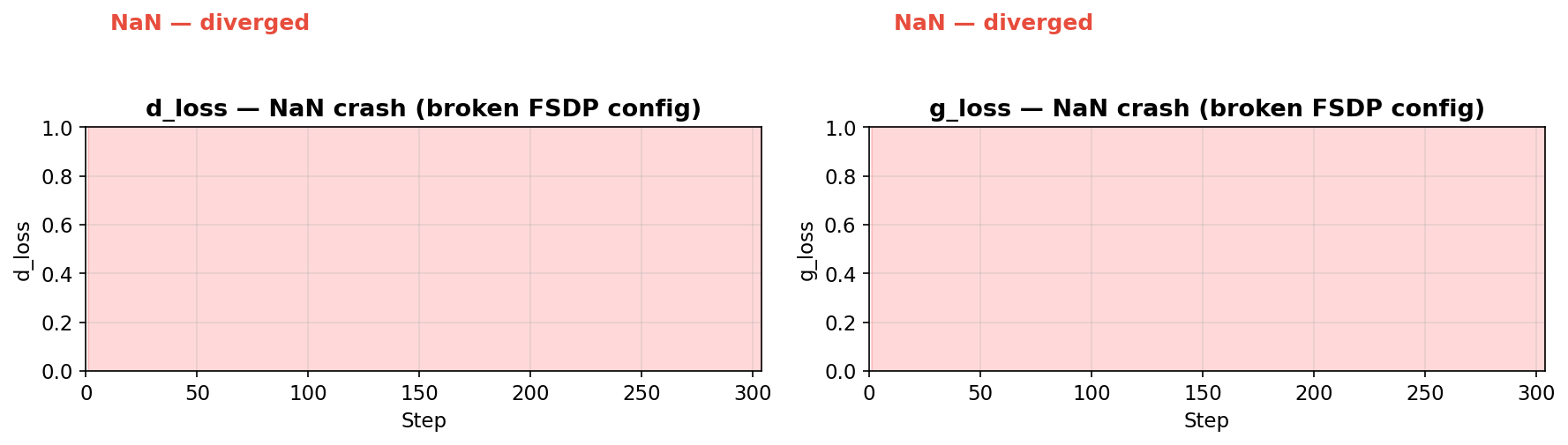
- NaN — training has diverged. Gradients exploded, likely from a broken FSDP config or incompatible optimizer settings. Example:
eager-smoke-151crashed at step 303 with NaN losses after we experimented with FSDP settings that broke gradient flow. Once NaN appears, the run is unrecoverable — kill it.
- d_loss pinned at 0 — discriminator is too confident on every sample. With batch_size=1, this is expected (hinge loss trivially saturates on a single sample). With batch_size≥2, it means the discriminator is dominating.
- g_loss flat and high — student isn’t improving despite non-zero d_loss. Check
grad_norm/student— if it’s zero on gen steps, the gradient path is broken.
Batch size effect on loss noise:
The per-step loss is computed on the micro-batch (per-GPU batch size), not the effective batch size. This has a dramatic effect on signal quality:
-
bs=1 (
vulcan-tanagra-110): Losses are extremely noisy — d_loss spikes between 0 and 4 every step, g_loss swings between -2 and 6. The hinge loss on a single sample is either fully saturated (0) or fully active — there’s no middle ground. This makes it very hard to tell from the loss curves alone whether training is progressing. -
bs=2 (
q1ft7t1z): Noticeably smoother. With 2 samples, the loss can take intermediate values (e.g. one sample saturated, one not = loss of ~1 instead of 0 or 4). The trends become readable.
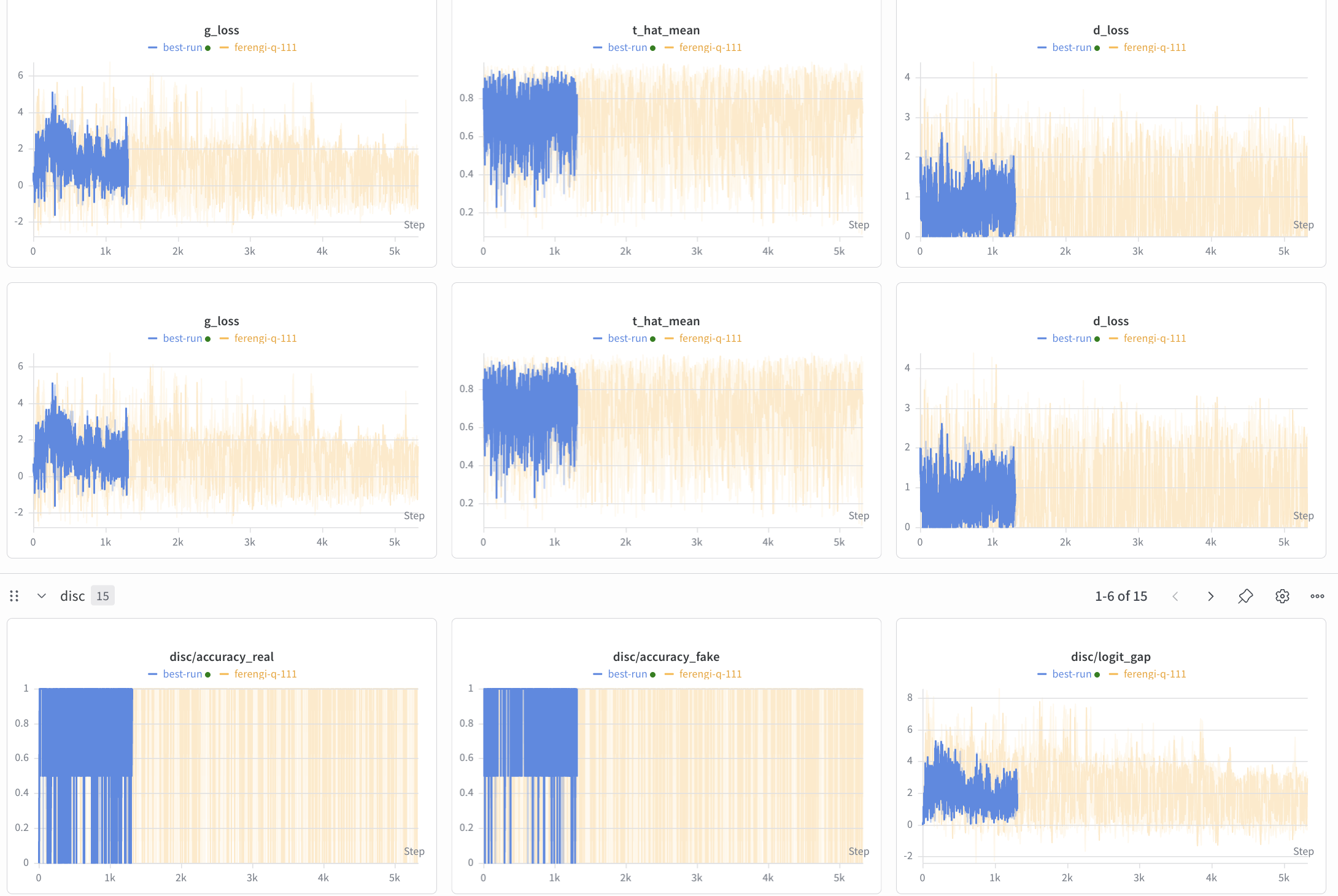
Here’s the W&B dashboard with both runs overlaid (blue = bs=2, orange = bs=1). The top row shows g_loss, t_hat_mean, and d_loss. The difference is stark — bs=2 (blue) has smoother loss curves with less oscillation, while bs=1 (orange) spikes violently between 0 and 4:
disc/accuracy_real and disc/accuracy_fake
How they’re computed (from ladd_eval.py:58-60):
accuracy_real = (real_logits > 0).float().mean()   # % of real samples classified as real
accuracy_fake = (fake_logits < 0).float().mean()   # % of fake samples classified as fake
These use a threshold of 0 (not the hinge margin of ±1). They measure whether the discriminator is directionally correct, even if not confident enough to produce non-zero loss.
Healthy range: Both between 0.6-0.9. The discriminator is right more often than not, but the student fools it sometimes.
Danger signs:
- Both pinned at 1.0 — discriminator dominance. Every sample is correctly classified with high confidence. The student gets no signal. This is what we saw in the collapsed full run with bs=1.
- Both below 0.5 at bs≥2 — discriminator has collapsed and can’t tell real from fake. The student gets random gradient directions. (At bs=1, accuracy of 0% on a single sample is normal — it just means the disc got that one sample wrong.)
- accuracy_real high but accuracy_fake low — discriminator learned to say “real” for everything. It correctly identifies real samples but can’t catch fakes.
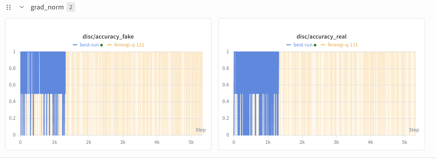
Important caveat: These are computed on the per-GPU micro-batch. With bs=1, accuracy can only be 0 or 1 — there are no intermediate values. With bs=2, it can be 0, 0.5, or 1. The zoomed-in accuracy view below makes this clear — bs=1 (orange) is binary, while bs=2 (blue) shows intermediate 0.5 values where the discriminator got one sample right and one wrong:
disc/logit_gap
How it’s computed:
logit_gap = real_logits.mean() - fake_logits.mean()
The raw difference between the discriminator’s average score on real vs fake samples. This is the most direct measure of how well the discriminator separates real from fake.
Healthy range: Positive and stable (2-6). The discriminator can tell them apart but isn’t overwhelmingly confident.
Danger signs:
- Logit gap > 15 — discriminator diverging, gradients likely exploding
- Logit gap < 0.1 — discriminator provides no learning signal, real and fake look identical to it
- Logit gap is NaN — training has diverged (same as NaN loss)
Per-layer logits (disc/layer_N_real, disc/layer_N_fake)
Each of the 6 discriminator heads (layers 5, 10, 15, 20, 25, 29) logs its own real/fake logit means. When all layers show nearly identical real and fake logits (as we saw in the collapsed run — layer_10_fake ≈ layer_10_real), it confirms the student outputs are indistinguishable from noise at every abstraction level.
Healthy training shows gaps at multiple layers, with late layers (25, 29) typically showing the largest gap (semantic-level discrimination is hardest to fool).
6. What We Observed
This section traces the full arc: from the untrained student baseline, through single-GPU validation, to the full cluster run — and the mode collapse that followed.
Untrained student baseline
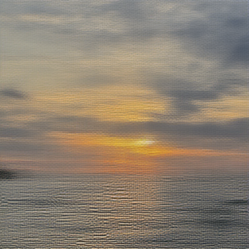
To understand how bad collapse can get, it helps to first see what the untrained student produces — teacher weights, 4 inference steps, zero LADD training (cerulean-cosmos-147):
| “Sunset over the ocean” | “Cat on a windowsill” | “Futuristic city skyline” | “Watercolor mountain landscape” |
|---|---|---|---|
 |
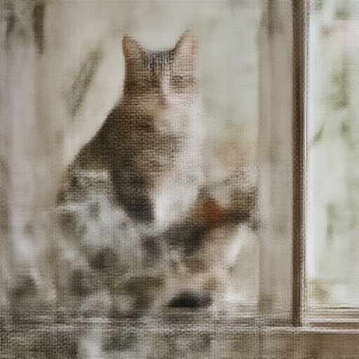 |
 |
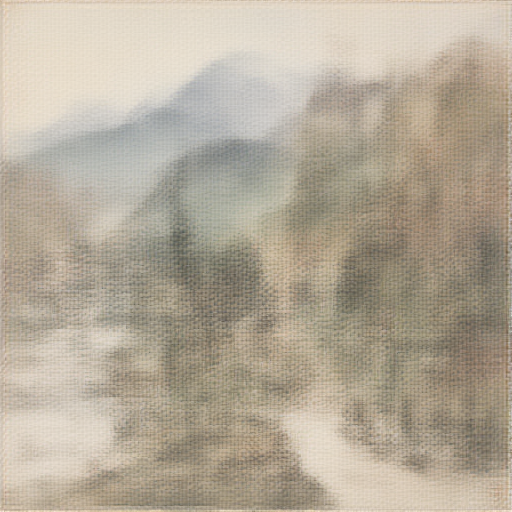 |
This is the floor — the student with teacher weights, no distillation training, producing images with just 4 steps. Anything LADD training does should improve upon this. The untrained baseline KID is 0.0689.
Single-GPU results
Here’s what the student produces at 4 steps compared to the teacher at 50 steps (CFG=5). These images are pulled directly from our W&B eval runs.
Prompt: “The image captures a dynamic scene at a bullfighting arena…“
| Teacher (50 steps, CFG=5) | Student (4 steps, 500 train steps) | Student (4 steps, 2000 train steps) |
|---|---|---|
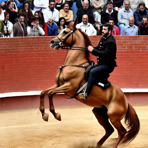 |
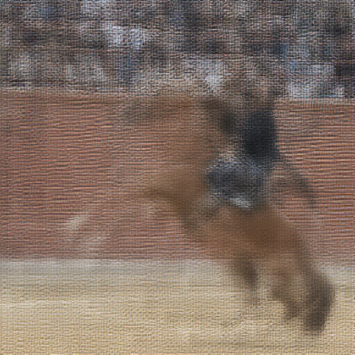 |
 |
Prompt: “cyberpunk birthday party with robots, androids and flamenco guitarist watching mars sunset…“
| Teacher (50 steps, CFG=5) | Student (4 steps, 500 train steps) | Student (4 steps, 2000 train steps) |
|---|---|---|
 |
 |
 |
Prompt: “The image displays a promotional advertisement for a speaker system. At the top of the image, in bold red letters…“
| Teacher (50 steps, CFG=5) | Student (4 steps, 500 train steps) | Student (4 steps, 2000 train steps) |
|---|---|---|
 |
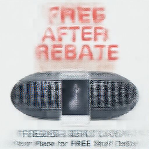 |
 |
This last example is the most encouraging — the student at 2000 steps picks up the layout (bold text, speaker image, URL at bottom) even though the details are still muddy. It shows the student is learning structure, just slowly at this tiny scale. This is expected: 500-2000 steps with batch_size=1 on 98 prompts is barely scratching the surface. The LADD paper uses 50K-200K steps with large batch sizes. The production 8-GPU run (20K steps, effective batch 64) should close this gap significantly.
Training progression
We tracked KID against 416 teacher-generated reference images (CFG=5, corrected scheduler) at different training checkpoints:
| Training steps | KID (↓ better) | d_loss | Observation |
|---|---|---|---|
| 500 | 0.0637 ± 0.0053 | 0.0 | Coarse structure emerges |
| 2000 | 0.0702 ± 0.0058 | 0.0 | KID worsens — disc collapse |
The KID worsening from 500 to 2000 steps was our first signal that something was off with the training dynamics. The discriminator loss collapsing to 0 at batch_size=1 meant the hinge loss saturated — the disc could perfectly separate real from fake with just 1 sample, providing no useful gradient.
This is expected at bs=1 and not a sign of discriminator dominance — the hinge margin of ±1 is trivially achieved with a single sample. At the production batch size of 64 (8 GPUs × 4 per-GPU × 2 grad accum), this saturation should resolve.
Overfit experiments
To verify the architecture itself works, we ran two overfit tests on just 10 prompts:
| Experiment | LR | Result |
|---|---|---|
| Aggressive (slr=1e-4, dlr=1e-3) | 20× higher | Diverged — pure noise output |
| Winning LR (slr=5e-6, dlr=5e-5) | Standard | Semantically correct but blue color shift |
The winning-LR overfit produced recognizable images matching prompts — proof that the gradient flow and architecture work. The blue color shift was mode collapse from tiny data: with 10 prompts and bs=1, the student oscillates between pleasing individual prompts instead of learning general features.
Key scaling evidence:
- Text conditioning works — compositions match prompts (98-prompt run)
- More data = better images (98 prompts > 10 prompts)
- More steps = better KID (500 steps: 0.00804 → 2000 steps: 0.00723, pre-fix)
- Gradient flow confirmed — weight deltas grow, grad norms are non-zero
- Discriminator active — d_loss oscillates, not collapsed
The bottleneck is compute and data scale, not architecture.
W&B run links
All experiments are tracked on W&B under project yeun-yeungs/ladd:
- v2 corrected training (500 steps)
- v2 eval at 500 steps
- v2 eval at 2000 steps
- v2 training at 2000 steps
Full cluster run: mode collapse at scale
We launched the first 8-GPU production run (yeun-yeungs/ladd/stjmyjsi) — 8x A100 80GB, 10K precomputed latents, 20K target steps. After all the single-GPU validation, FSDP debugging, and hyperparameter sweeps, this was supposed to be the payoff run.
The results were devastating.
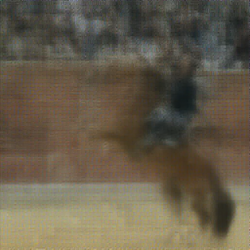
Here’s what 1000 steps of single-GPU training (bs=1, 98 debug prompts) produces — blurry but with correct structure (rqn4r0sg, equivalent to ~125 steps on 8 GPUs):
| “Bullfighting arena” | “Wine bottles” | “Cyberpunk party” | “Man with logos” |
|---|---|---|---|
 |
 |
 |
 |
These are blurry but recognizable — the student starts from a reasonable place and single-GPU training does improve structure. LADD training on the full cluster is supposed to make these sharper. Instead, it destroyed them:
By step 2000, all outputs collapse into the same colorful noise pattern regardless of prompt:
Prompt: “A row of colorful, stylized, and simplified animal figures…“
| Teacher (50 steps) | Student step 0 | Student step 2000 | Student step 4000 |
|---|---|---|---|
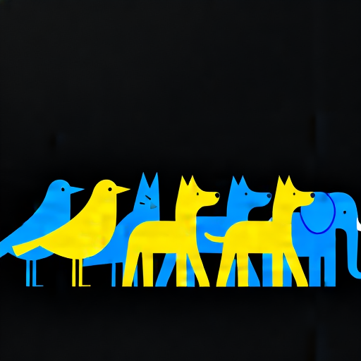 |
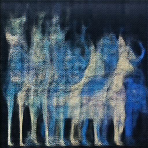 |
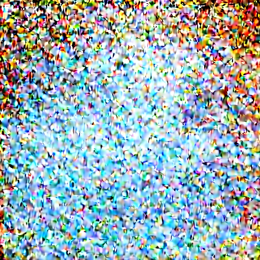 |
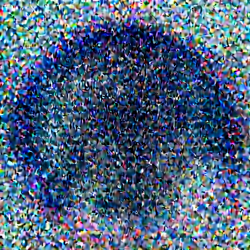 |
Prompt: “videogame screenshot of a very psychedelic dreamy luxury flooded tropical universe…“
| Teacher (50 steps) | Student step 0 | Student step 2000 | Student step 4000 |
|---|---|---|---|
 |
 |
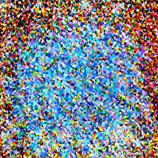 |
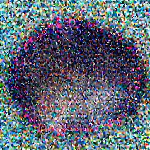 |
Every prompt produces the same speckled noise. The KID at step 4000: 0.593 — catastrophically high. For reference, the untrained student (teacher weights, zero LADD training) scores KID = 0.069. Training didn’t just fail to improve — it made the model 8.6× worse than not training at all.
The full degradation timeline
The gallery below tracks 4 prompts across 12 checkpoints (every 500 steps from step 500 to step 6000). At step 500 there’s still recognizable structure from the teacher-initialized weights. By step 1000-1500 the images start losing coherence. From step 2000 onward, every prompt produces the same speckled noise — the student has fully collapsed.
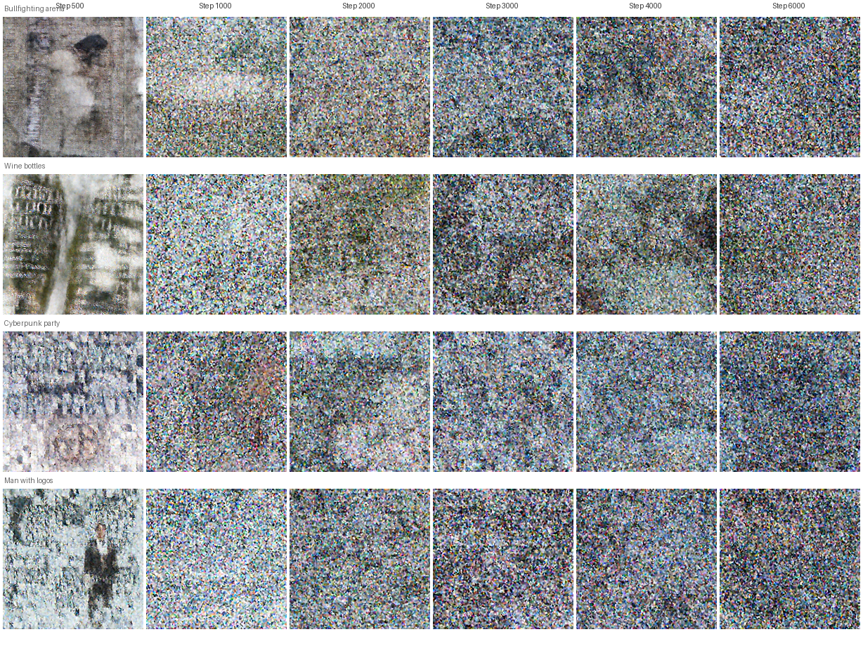
The uniformity of the collapsed outputs across completely different prompts (bullfighting arena, wine bottles, cyberpunk party, man with logos) confirms this is mode collapse, not just poor quality — the student is producing a single “average” output regardless of conditioning.
Eval images from yeun-yeungs/ladd-eval.
Learning curves from W&B
We tracked two production runs on the 8-GPU cluster (zzu1qpx4 and ciiv9vjy), both bs=2 with renoise_m=1.0. The KID curve tells the full story — training consistently makes the model worse:
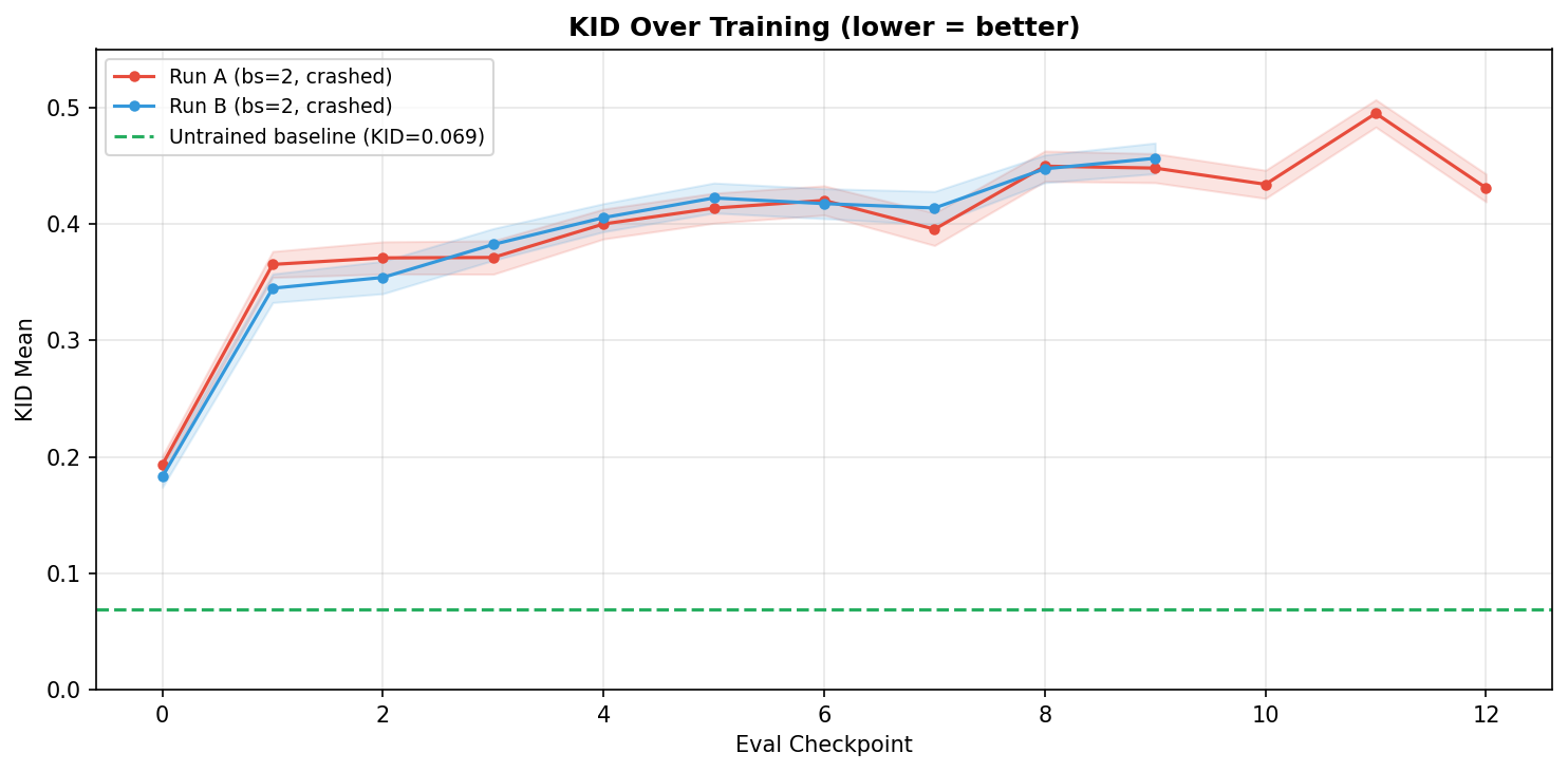
The untrained student (green dashed line, KID=0.069) is better than every single training checkpoint. KID climbs from 0.19 at the first eval to 0.45-0.50 by the end — the student is actively un-learning.
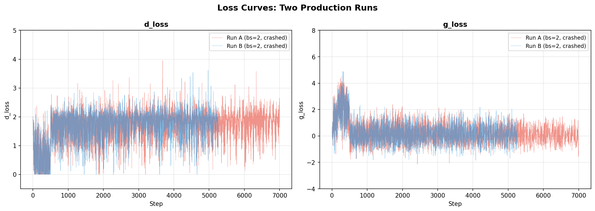
The loss curves show the adversarial dynamics aren’t converging:
The discriminator health metrics reveal the underlying problem — the logit gap collapses toward zero over time, meaning the discriminator gradually loses its ability to distinguish real from fake:
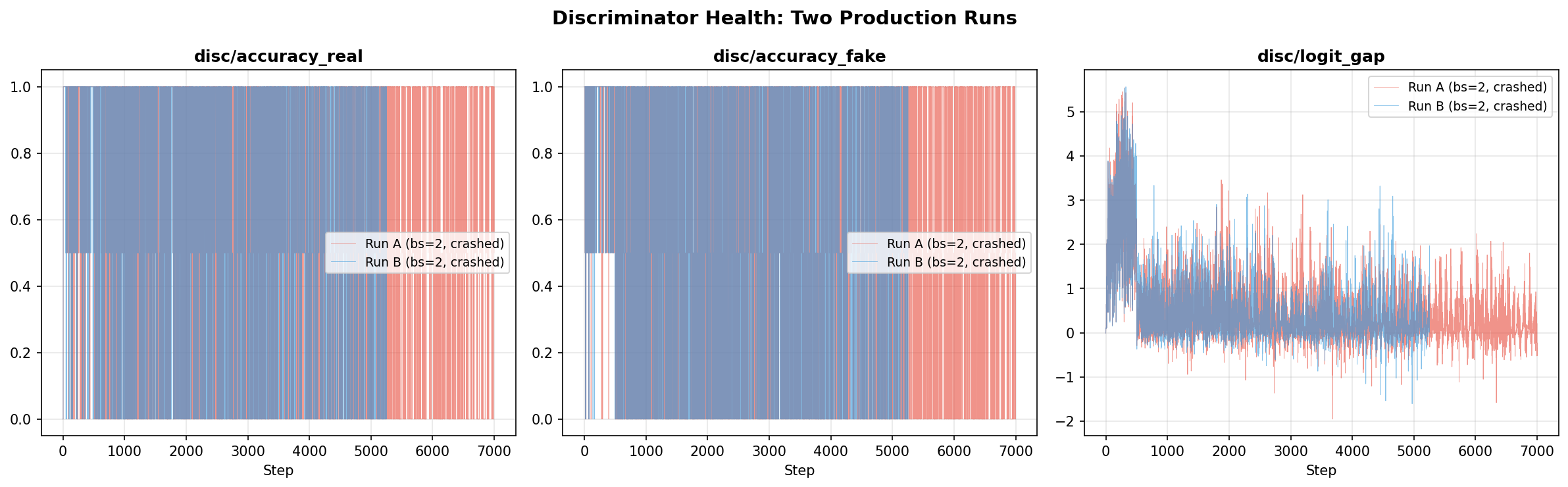
Root cause analysis
The discriminator accuracy charts told a misleading story — disc/accuracy_real and disc/accuracy_fake both pinned at 1.0 throughout training. At first glance, this screamed “discriminator too strong, student getting no gradient.”
But d_loss and g_loss were actually non-zero and oscillating (0-4 range). The losses existed — so why wasn’t the student learning?
The answer: the accuracy was computed on a per-GPU micro-batch of 1 sample. With batch_size=1, the discriminator trivially classifies one sample. The accuracy metric was degenerate, not the training signal itself. We needed to look at the loss curves, not the accuracy.
The production run diverged from our validated best config in two critical ways:
| Parameter | Production run | Validated best | Impact |
|---|---|---|---|
train_batch_size |
1 | 2-4 | Hinge loss on 1 sample saturates to 0 every micro-step. Gradient accumulation sums 8 zeros = zero. |
renoise_m |
1.0 | 0.5 | Discriminator mostly sees heavily noised samples (sigmoid(1.0)=0.73). Gradient signal is weak even when non-zero. |
The combination was lethal: weak gradients from high-noise re-noising (m=1.0), further zeroed out by degenerate hinge loss on single samples. The student drifted from its teacher-initialized weights into noise with no corrective signal.
The fix
--train_batch_size=2              # was 1 — hinge loss needs >1 sample
--gradient_accumulation_steps=4   # was 8 — keeps effective BS=64 (2×4×8)
--renoise_m=0.5                   # was 1.0 — 43% better in sweep
--warmup_schedule_steps=0         # was 10 — no benefit in sweep
Lesson: The total effective batch size is not the only thing that matters — the per-micro-step batch size determines whether the loss function produces meaningful gradients. Hinge loss with bs=1 is degenerate. And always double-check that production configs match your validated sweep winners.
Qwen vs CLIP embeddings for discriminator conditioning
We initially used mean-pooled Qwen self-attention features for the discriminator’s FiLM conditioning. Switching to CLIP embeddings gave the discriminator a stronger semantic signal. Interestingly, KID results were similar between the two — the CLIP version’s main benefit was that renoise_m=1.0 became optimal (the discriminator could discriminate even at higher noise levels), simplifying the hyperparameter search.
7. Technical Difficulties
Two major bottlenecks consumed the most debugging time: data preprocessing constraints and distributed training issues.
Data preprocessing bottleneck
We had 500K curated prompts but needed teacher latents (50-step generation with CFG=5) for every one. With 6 hours of compute, we could precompute roughly 10K latents in 4 hours — 2% of our dataset. Training would repeat each latent ~128 times over 20K steps.
This was a hard trade-off we should have modeled before curating 500K prompts. The curation pipeline (Part 1) was optimized for diversity and prompt quality, which is still valuable for future runs. But for the first training run, 10K stratified-sampled prompts with heavy repetition was the reality.
The 10K subset overfits quickly — KID degrades after 500 steps on 3K data, and the full 10K was not large enough for the 20K-step production run either.
Scaling up: the FSDP journey

Why FSDP?
On a single A100 80GB, the memory budget is brutal:
| Component | Size |
|---|---|
| Student (bf16) | 12 GB |
| Teacher (bf16) | 12 GB |
| Student optimizer (fp32 Adam) | 24 GB |
| Activations (512px, grad ckpt) | ~30 GB |
| Total | ~78 GB → OOM |
We first tried 8-bit Adam (bitsandbytes) to cut optimizer states from 24 GB to 6 GB. This worked at 256px but still OOM’d at 512px due to activation memory. The real solution was multi-GPU.
DeepSpeed: 9 ways to fail
Before FSDP, we tried DeepSpeed ZeRO-2 with CPU optimizer offload. It failed in 9 distinct ways — each one a lesson in why DeepSpeed assumes single-model training:
- Dual engine crash — wrapping both student and discriminator caused
IndexErrorin gradient reduction - Two-Accelerator pattern — failed with
mpi4pyerrors on seconddeepspeed.initialize() - Student LR stuck at 0 — DeepSpeed’s internal WarmupLR didn’t configure correctly through Accelerate’s “auto” values
- Frozen disc broke gradient flow —
discriminator.requires_grad_(False)during gen step severed the computation graph, student grad norms were zero - Double gradient reduction — both
d_loss.backward()andg_loss.backward()triggered ZeRO-2’s reduction hooks on student params - Grad norms always zero — captured after
zero_grad(); ZeRO-2 manages gradients in internal buffers - Checkpoint write failure —
PytorchStreamWriter failedon the ~24GB optimizer state file os.execv+teeincompatibility — experiment runner output not captured- GPU memory leak via
fork()— parent process held GPU memory, child OOM’d
Conclusion: DeepSpeed ZeRO is designed for single-model training. The GAN setup with alternating D/G updates, cross-model gradient flow, and two optimizers is fundamentally incompatible.
FSDP configuration
FSDP (Fully Sharded Data Parallel) worked cleanly because it operates at the module level rather than the optimizer level. Our config wraps each of the 30 transformer blocks as separate FSDP units:
From training/fsdp_config.yaml:
fsdp_config:
  fsdp_auto_wrap_policy: TRANSFORMER_BASED_WRAP
  fsdp_transformer_layer_cls_to_wrap: ZImageTransformerBlock
  fsdp_sharding_strategy: FULL_SHARD
  fsdp_backward_prefetch: BACKWARD_PRE
  fsdp_use_orig_params: true      # Required for per-param optimizer groups
  fsdp_state_dict_type: FULL_STATE_DICT
Key design choice: the teacher is NOT wrapped in FSDP — it’s replicated on every GPU. At 12 GB in bf16, it fits easily on 80GB A100s, and it only does forward passes (no optimizer states to shard). Wrapping it would add FSDP all-gather overhead for no memory benefit.
Memory per GPU with FSDP
| Component | Per-GPU Size |
|---|---|
| Student (sharded 1/8) | ~1.5 GB |
| Student optimizer (sharded 1/8) | ~6 GB |
| Teacher (full replica) | ~12 GB |
| Discriminator | ~0.03 GB |
| Activations + grad checkpointing | ~4-6 GB |
| Total | ~26 GB / 80 GB |
Comfortable margin. No need for 8-bit Adam, CPU offloading, or precomputed text embeddings on the cluster.
FSDP debugging issues
The get_state_dict hang: FSDP’s accelerator.get_state_dict() is a collective operation — all ranks must call it, not just rank 0. Our validation code called it inside an if accelerator.is_main_process: guard. Rank 0 entered the gather; ranks 1-7 skipped it. Deadlock.
From the fix in train_ladd.py:263:
# get_state_dict is a collective op under FSDP — ALL ranks must call it.
state_dict = accelerator.get_state_dict(student_model)

# Only rank 0 does file I/O
if not accelerator.is_main_process:
    return
Checkpoint format issues: accelerator.save_state() is incompatible with 8-bit Adam under FSDP. PyTorch’s .pt format had temp file issues with large state dicts. The fix: save student weights as safetensors, gate save_state behind if not is_fsdp.
Validation subprocess can’t log to parent’s W&B: Our async validation spawns a subprocess on a separate GPU. The child process can’t resume the parent’s W&B run context. Fix: the parent process logs the eval table after the subprocess completes.
The costly get_state_dict double-call: get_state_dict() takes ~10 minutes for FSDP gather on a 6B model. We were calling it separately for checkpointing and validation — 20 minutes wasted when they coincide at the same step. Fix: one call, shared between both.
if need_checkpoint or need_validation:
    state_dict = accelerator.get_state_dict(student)  # Single gather
    if need_checkpoint:
        save_checkpoint(state_dict)
    if need_validation:
        launch_validation(state_dict)
8. Lessons Learned
We made mistakes that cost days of debugging and invalidated entire experiment rounds. These are the principled takeaways.
Validate your baseline before tuning anything
We ran 21 hyperparameter experiments and found a configuration that scored KID = 0.000869 — an 89% improvement over baseline. Then we discovered five critical bugs in the training pipeline, and every single KID number became meaningless.
Bug 1: Scheduler linspace off-by-one
Our custom FlowMatchEulerDiscreteScheduler.set_timesteps() had a subtle indexing error:
# BROKEN — leaves 11% residual noise at the final step
timesteps = np.linspace(sigma_max_t, sigma_min_t, num_inference_steps + 1)[:-1]

# CORRECT — matches diffusers exactly
timesteps = np.linspace(sigma_max_t, sigma_min_t, num_inference_steps)
With 50 inference steps, the scheduler’s smallest sigma was 0.109 instead of reaching 0.0. Teacher images had 11% residual noise — they looked blurry, and we were evaluating KID against blurry references.
Bug 2: Teacher images generated without CFG
The precompute_fid_reference.py script generated teacher reference images with guidance_scale=0. The Z-Image model requires CFG (~5.0) for sharp, well-composed images. Without it, outputs were unconditional-like and lacked detail. On top of that, TeaCache was enabled (teacache_thresh=0.5), skipping 75% of transformer computations for speed at the cost of further quality degradation.
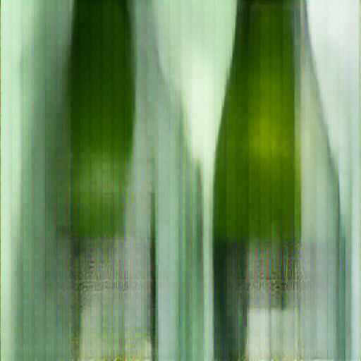
The difference is stark — here’s the same prompt rendered with CFG=0 vs CFG=5 (from our W&B debug-teacher-cfg-sweep run):
Prompt: “Two wine bottles with green glass and white labels…“
| CFG=0 (no guidance) | CFG=3 | CFG=5 (selected) |
|---|---|---|
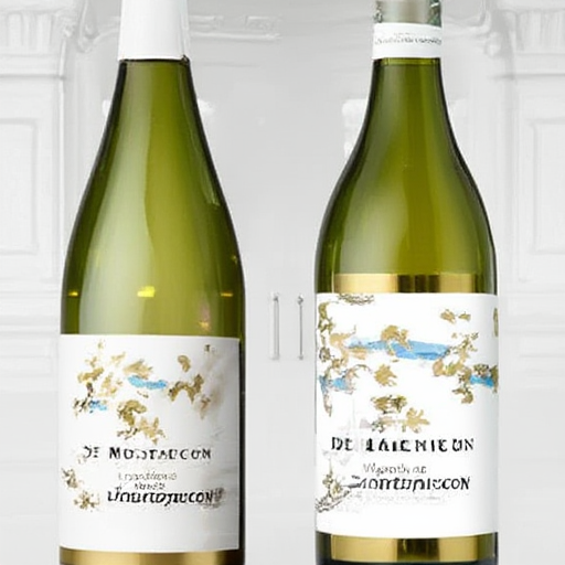 |
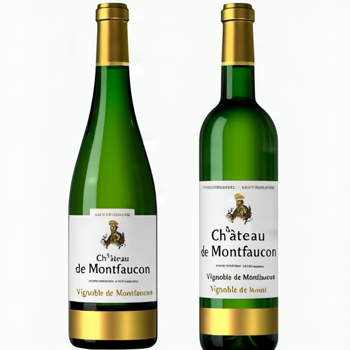 |
 |
Without CFG, the labels are illegible smudges. With CFG=5, the text is crisp and the bottle shapes are well-defined. We were evaluating our student against the left image — no wonder the KID numbers looked deceptively good.
Bug 3: Student input was pure noise regardless of timestep
The student at timestep $t = 0.25$ should see a mostly-clean input: $x_t = 0.75 \cdot x_0 + 0.25 \cdot \varepsilon$. Instead, it received pure noise at every timestep. At $t = 0.25$, the student was told “you’re almost done denoising” while looking at pure static — it had no signal about what to reconstruct.
Bug 4: No velocity-to-latent conversion
The student predicts velocity $v_\theta$, but the code used raw velocity as the denoised prediction. The correct conversion is $\hat{x}0 = x_t - t \cdot v\theta$ — without it, the discriminator received meaningless inputs.
Bug 5: “Real” samples were noise vs. noise
The LADD paper (Section 3.2) specifies that “real” samples should be teacher-generated images re-noised to the discriminator’s timestep. Our code used add_noise(noise1, noise2, t_hat) — random noise mixed with random noise. The discriminator was learning to distinguish two flavors of Gaussian noise, which is a trivially learnable but useless task.
The corrected training flow:
OFFLINE:
  teacher_x0 = teacher.generate(prompt, cfg=5, steps=50, output_type="latent")

ONLINE per step:
  1. x_t = (1-t) * teacher_x0 + t * ε           ← student input (Bug 3 fix)
  2. v = student(x_t, t, prompt)                  ← velocity prediction
  3. x̂_0 = x_t - t * v                           ← denoised latent (Bug 4 fix)
  4. fake_noisy = (1-t̂) * x̂_0 + t̂ * ε₁           ← re-noise for disc
  5. real_noisy = (1-t̂) * teacher_x0 + t̂ * ε₂     ← real path (Bug 5 fix)
The worst part: the relative ordering of hyperparameter configs from Round 1 likely still holds (all experiments used the same broken pipeline), but the optimal GI flipped from 8 to 3 once the discriminator faced a genuinely hard discrimination task. We had to re-run the entire sweep.
Principle: Never tune hyperparameters on an unvalidated baseline. Before any sweep, verify: (1) the teacher produces sharp images independently, (2) the training loop’s math matches the paper step-by-step, (3) a single training step produces finite, non-trivial gradients. Log teacher outputs to W&B as a sanity check before starting experiments.
Instrument first, debug later
Several of our bugs were only caught because we logged the right things to W&B — and several persisted because we didn’t log the right things early enough.
What caught the scheduler bug: We logged teacher images to W&B as part of a CFG sweep (debug-teacher-cfg-sweep). The images looked blurry at all CFG values. This prompted investigation of the scheduler, which revealed the linspace off-by-one. Without visual inspection, we would have continued tuning hyperparameters against a broken baseline.
What we should have logged earlier:
- Teacher-generated images at step 0 (before any training)
- The exact timestep and sigma values the scheduler produces
- A side-by-side of student input $x_t$ at different timesteps (would have caught Bug 3 immediately — “why does t=0.25 look like pure noise?”)
- Decoded student predictions $\hat{x}_0$ (would have caught Bug 4 — raw velocity doesn’t look like an image)
The pixelated artifact investigation: Student outputs showed pixelated grid artifacts. The investigation led us to the scheduler parameters, which led to the linspace bug. The fix required regenerating all teacher reference images and latents, then re-running every experiment.
Principle: Log intermediate representations, not just scalar metrics. Scalars like KID and d_loss tell you that something is wrong; images and tensors tell you what. At minimum, log: teacher outputs at step 0, student predictions every N steps, input $x_t$ at different timesteps, and scheduler sigma schedules. A 5-minute W&B setup saves days of blind debugging.
Debug slices lie
All 21 hyperparameter experiments ran on a 98-prompt debug slice with train_batch_size=1 on a single GPU. The sweep converged, KID improved, the architecture was validated. We were confident.
Then we launched the full 8-GPU run with 10K prompts — and the student collapsed into noise within 2000 steps (Section 6).
The debug slice succeeded for the wrong reasons:
- bs=1 with 98 prompts: each prompt was seen every ~98 steps. The student effectively memorized the discriminator’s feedback on specific prompts. The hinge loss saturated on individual samples, but the rapid prompt cycling created enough gradient diversity to mask the problem.
- Scaling to 10K prompts: each prompt seen every ~10K steps. The student no longer cycles through familiar prompts fast enough to maintain that implicit diversity. The degenerate bs=1 hinge loss becomes the dominant dynamic, and the student drifts.
- Config drift: the production run accidentally used
renoise_m=1.0andwarmup_schedule_steps=10instead of the validated0.5and0. The debug sweep validated one config; the production run launched a different one. No automated check caught the mismatch.
The fix required increasing train_batch_size from 1 to 2 (so the hinge loss is non-degenerate per micro-step) and ensuring the production config exactly matched the sweep winners.
Principle: Your debug slice is not a miniature version of your full run — it’s a different problem. Validate on the debug slice to confirm the architecture works, but expect hyperparameters to shift at full scale. At minimum: (1) test with a realistic per-GPU batch size before launching, (2) diff your production launch command against your best sweep config, and (3) add validation image logging from step 0 so you catch collapse immediately instead of discovering it hours later.
9. Summary & Next Steps
What we built
A LADD training framework that distills a 6.15B parameter image model from 50 inference steps to 4:
- Architecture: Student (6.15B, trainable) + Teacher (6.15B, frozen) + Discriminator (14M, 6 multi-scale conv heads on teacher features, CLIP-conditioned)
- Loss: Adversarial hinge loss only — no distillation loss, no pixel-space comparison
- Training: Asymmetric D/G updates (3:1), logit-normal re-noising ($m=1.0$, $s=1.0$), timestep curriculum
- Infrastructure: FSDP across 8× A100 80GB, precomputed teacher latents and text embeddings, W&B logging
What we learned
Our experimental methodology followed a clear pipeline:
- Precompute all latents and embeddings offline (teacher latents with CFG=5, Qwen text embeddings, CLIP embeddings for disc conditioning)
- Small runs on 3K data subsets with a single A100 to test hypotheses — 500 steps each, measuring KID against teacher reference images, keeping only configs that beat the untrained baseline (KID = 0.069)
- Launch the best config on the full 8-GPU cluster
Key findings from three rounds of sweeps (33+ experiments):
- GI=3 is consistently optimal across all architecture versions
- Disc LR should be modest (1e-5, not 5e-5) — the discriminator doesn’t need to be aggressive
- Batch size > 1 is critical — hinge loss with bs=1 is degenerate (zero gradient per micro-step)
- bs=2 vs bs=1 dramatically stabilizes training — smoother loss curves, non-trivial accuracy, less oscillation
- Run-to-run variance is high at 500 steps / bs=1: a single “best” run can be 2× better than the true mean. Always run 3-5 seeds.
- 1000 steps overfits on 3K data — more data (10K+) is needed before longer training helps
- Qwen vs CLIP embeddings for disc conditioning: switching to CLIP embeddings gave the discriminator a stronger semantic signal. KID results were similar, but the CLIP version simplified the hyperparameter search by making
renoise_m=1.0optimal.
What went wrong
- Data preprocessing bottleneck: precomputing teacher latents at ~7s/image limited us to 10K of our 500K prompts. The 10K subset overfits quickly — KID degrades after 500 steps.
- Mode collapse on the full cluster run: misconfigured hyperparameters (
bs=1+renoise_m=1.0instead of validated config) caused the student to collapse into noise within 2000 steps. KID went from 0.069 (untrained) to 0.593 (8.6× worse). - FSDP debugging: collective operation hangs, checkpoint format incompatibilities, subprocess W&B logging failures, and 10-minute
get_state_dictcalls — each consumed hours. - Config drift: debug sweep validated one config, production launched a different one. No automated check caught the mismatch.
What to try next
- More fine-grained evaluation — run KID at every 500 steps out to step 4000+ to get more signal on the degradation curve and identify the optimal early-stopping point
- Higher batch size (bs=4+) for more stable gradient flow — requires memory optimization (activation checkpointing, offloading) to fit on A100 80GB
- Alternative loss functions — variants of the GAN loss (non-saturating loss, Wasserstein loss, R1 gradient penalty) may provide more stable gradients than hinge loss, especially at small batch sizes
- EMA (Exponential Moving Average) weight updates — maintain a running average of student weights to smooth out oscillations during adversarial training. A common GAN stabilization technique we haven’t explored yet.
- Scale up training data — precompute latents for 50K+ prompts to reduce overfitting and enable longer training runs
- Multi-seed averaging — run 3-5 seeds per config and report mean KID to avoid false confidence from lucky single runs
The code is open source at github.com/vionwinnie/Z-Image-LADD-distillation.
10. Appendix: Anti-Mode-Collapse Sweep
After the first full run collapsed (Section 6), we ran a second round of experiments specifically targeting discriminator dominance. The goal: find hyperparameters that prevent mode collapse on the full 10K dataset. Reference untrained KID: 0.0689 (anything above means training made things worse).
The Phase 1 sweep results (debug split, 98 prompts) are covered in Section 4. For reference, the untrained student (teacher weights, no LADD training at all) has KID = 0.0689 ± 0.0067 at 4 inference steps. Any KID above this means training actively made things worse.
This appendix covers Phase 2 — the anti-collapse sweep run after the production failure, using a fresh evaluation setup with corrected teacher images:
| Run | Config | KID | Verdict |
|---|---|---|---|
| GI=2, dlr=1e-5 | weaker disc | 0.0666 | Best in this phase (below untrained baseline) |
| GI=2, dlr=1e-5, dim=128 | even weaker | 0.0664 | Best overall in Phase 2 |
| GI=2, dlr=2e-5 | 0.0684 | Slightly worse | |
| GI=3, dlr=1e-5 | 0.0728 | Worse | |
| GI=2, dlr=1e-5, dim=128, layers=[10,20,29] | two changes at once | 0.0791 | Worse |
| Last run | slr=5e-6, dlr=1e-5, gi=2 | 0.0788 | Regression (KID above untrained baseline) |
Takeaways from the sweep
-
GI is the dominant knob. Phase 1: GI=3→8 gave 89% improvement. Phase 2: GI=2 with low disc LR was the sweet spot. The optimal value depends on the evaluation regime.
-
Lower disc learning rate helps.
dlr=1e-5consistently outperformeddlr=5e-5at preventing discriminator dominance. -
Smaller disc hidden dim has diminishing returns.
dim=128helped marginally;dim=512hurt badly. The default 256 is a reasonable middle ground. -
Noise schedule (renoise_m) matters less than GI.
M=0.5was best, but the effect was modest compared to GI tuning. -
Disc layer indices didn’t help. Reducing from 6 to 3 or expanding to 8 layers always made things worse.
-
The sweet spot is narrow. The discriminator must be strong enough to provide signal but not so strong that it overwhelms the student. This fundamental tension in adversarial distillation makes hyperparameter tuning particularly sensitive — small changes in GI or disc LR can flip between the two failure modes.
11. Key References
| Year | Paper | Contribution |
|---|---|---|
| 2023 | Lipman et al., Flow Matching for Generative Modeling | Flow matching framework — linear interpolation between noise and data, velocity prediction |
| 2023 | Sauer et al., Adversarial Diffusion Distillation (ADD) | First adversarial distillation for diffusion — SDXL-Turbo, 1-4 step generation |
| 2024 | Sauer et al., LADD: Latent Adversarial Diffusion Distillation | Moves discrimination to teacher’s latent features — scalable, no pixel losses, 14M discriminator for 6B+ models |
| 2018 | Miyato et al., Spectral Normalization for GANs | Hinge loss and spectral norm — stabilizes adversarial training |
| 2018 | Perez et al., FiLM: Visual Reasoning with Feature-wise Linear Modulation | FiLM conditioning — scale/shift modulation used in discriminator heads |