LADD Distillation: What Worked, What Broke, What's Next
April 7, 2026
This is a self-contained summary of our LADD distillation project – distilling a 6.15B parameter text-to-image model from 50 inference steps down to 4. Think of it as the conference talk version of a longer paper: what we built, what we learned, and what broke.
For the full technical deep-dive with all the code and W&B screenshots, see Part 2: Training Framework. For the data curation pipeline, see Part 1: Data Curation.
Code: github.com/vionwinnie/Z-Image-LADD-distillation
tl;dr: We built a LADD training framework, ran 33+ experiments to find the best hyperparameters, and launched on an 8-GPU cluster. The architecture works – single-GPU experiments showed clear improvement. But the production run mode-collapsed due to a degenerate batch-size-1 hinge loss combined with config drift. The fix is known (bs>=2, match validated config), but our compute budget ran out before we could rerun.
1. What is LADD?
Latent Adversarial Diffusion Distillation (Sauer et al., 2024) is a method for making diffusion models faster. Instead of minimizing MSE between teacher and student outputs (which produces blurry images), LADD uses adversarial training – a GAN – operating in the teacher’s latent feature space. A lightweight discriminator learns to distinguish teacher features from student features, and the student learns to fool it.
The setup involves three models:
| Component | Parameters | Role | Trainable |
|---|---|---|---|
| Student (S3-DiT) | 6.15B | Denoises in fewer steps | Yes |
| Teacher (S3-DiT) | 6.15B | Provides feature representations | No (frozen) |
| Discriminator (Conv heads) | 14M | Multi-scale adversarial feedback | Yes |
The student is initialized as an exact copy of the teacher. Training teaches it to skip steps – to produce in 4 steps what the teacher produces in 50. The discriminator is tiny (0.2% of the student) because it only needs to classify features, not generate images. There are also two frozen encoders in the pipeline: a Qwen3 text encoder (~3B) for prompt conditioning and a VAE (~0.5B) for converting between latent and pixel space.
The key insight of LADD over earlier adversarial distillation (ADD) is that discrimination happens in the teacher’s latent feature space, not pixel space. The frozen teacher’s intermediate transformer activations become the comparison signal. This is what makes a 14M discriminator sufficient for a 6B model – it operates on rich, pre-extracted features rather than raw pixels.

2. The Core Mechanism
The training loop has four moving parts: timestep sampling, student velocity prediction, re-noising for discriminator comparison, and asymmetric updates. Here is how they fit together.
Flow matching velocity prediction
Unlike noise-prediction diffusion models (DDPM), Z-Image uses flow matching (Lipman et al., 2023) where the forward process interpolates linearly between data and noise:
\[x_t = (1 - t) \cdot x_0 + t \cdot \varepsilon\]Here $x_0$ is the clean teacher latent (generated with CFG=5 over 50 steps), $\varepsilon$ is Gaussian noise, and $t \in [0, 1]$ is the timestep (higher = noisier). The student predicts a velocity $v_\theta$ and we recover the denoised latent:
\[\hat{x}_0 = x_t - t \cdot v_\theta(x_t, t, c)\]where $c$ is text conditioning from the Qwen3 encoder. In code: student_pred = x_t - t_bc * student_velocity.
Re-noising for fair comparison
The student’s prediction and the teacher’s clean latent can’t be compared directly – the student just started training, so its outputs are worse for trivial reasons. Instead, both are re-noised to a shared noise level $\hat{t}$, sampled from a logit-normal distribution. The logit-normal applies a sigmoid to a Gaussian sample, concentrating values in $(0, 1)$ away from the extremes. This creates a fair comparison space where the discriminator sees a smooth mix of noise levels:
def logit_normal_sample(batch_size, m=1.0, s=1.0, device="cpu", generator=None):
    """Sample from logit-normal: u ~ Normal(m, s^2), t = sigmoid(u)."""
    u = torch.normal(mean=m, std=s, size=(batch_size,), generator=generator, device=device)
    t = torch.sigmoid(u)
    t = t.clamp(0.001, 0.999)
    return t
Hinge loss
The adversarial signal comes from a hinge loss – the same loss used in spectral normalization GANs. It has a nice property: the discriminator loss saturates once confident, preventing it from becoming arbitrarily strong.
d_loss = torch.mean(F.relu(1.0 - real_logits)) + torch.mean(F.relu(1.0 + fake_logits))
g_loss = -torch.mean(fake_logits)
The discriminator pushes real logits above +1 and fake logits below -1. Once confident, the ReLU clips to zero – no further gradient, preventing the discriminator from running away. The student simply maximizes its own logits.
A critical design choice: the student updates only every $N$ discriminator steps (gen_update_interval), keeping the discriminator ahead. The discriminator also uses a higher learning rate (typically 2-10x the student’s). If both update every step at the same rate, they oscillate destructively.
One subtle but essential detail: gradients flow through the frozen teacher. The teacher’s weights are frozen (requires_grad_(False)), but on the fake path, the computation graph is kept alive – no torch.no_grad(). This means gradients backpropagate through the teacher’s forward operations to reach the student.
The discriminator itself is 6 independent lightweight convolutional heads, each attached to a different layer of the teacher transformer (layers 5, 10, 15, 20, 25, 29). Early layers capture texture and local patterns; middle layers capture object composition; late layers capture semantics and prompt alignment. If the discriminator only watched one layer, the student could learn to fool that specific abstraction level while degrading at others. Six layers make gaming the system much harder.
Each head uses FiLM conditioning (Feature-wise Linear Modulation) from the timestep and CLIP text embedding, so the discriminator adjusts which features matter depending on the noise level and prompt content. The student also sees a timestep curriculum: during warmup, it trains on easy tasks (low noise). After warmup, 70% of samples are at $t = 1.0$ (full denoising from pure noise) – the hardest case and what matters most for 4-step inference. The asymmetric update schedule in code:
is_gen_step = (global_step % args.gen_update_interval == 0)

# Discriminator: always update
accelerator.backward(d_loss)
disc_optimizer.step()

# Student: update every N steps
if is_gen_step:
    accelerator.backward(g_loss_update)
    student_optimizer.step()

3. Experimental Setup
Our pipeline had four stages:
Stage 1: Precompute. Teacher latents (50-step generation, CFG=5) + Qwen text embeddings + CLIP embeddings for all training prompts, computed offline. The teacher generates a clean latent for each prompt, which becomes both the training target and the “real” sample for the discriminator. We benchmarked throughput:
| Batch size | Time per image | Peak VRAM |
|---|---|---|
| 1 | 8.9s | 21.9 GB |
| 4 | 7.5s | 25.2 GB |
| 8 | 7.3s | 29.5 GB |
At 7.3s per image with embarrassingly parallel sharding across 8 GPUs, precomputing all 500K latents would take ~127 hours. We had 6 hours. The math was brutal: we could precompute roughly 10K latents in 4 hours – just 2% of our 500K curated prompts. This was our biggest constraint: we had carefully curated 500K diverse prompts (Part 1) but could only use 10K for training. Each latent would be repeated ~128 times over 20K steps.
Stage 2: Small-run sweeps. 500-step experiments on 3K data subsets, single A100 80GB. Evaluated with KID (Kernel Inception Distance) – an unbiased metric preferred over FID for small sample sizes. Lower is better. The untrained student (teacher weights, zero training) scored KID = 0.069. We kept only configs that beat this baseline.
Stage 3: Autoresearch framework. Inspired by Karpathy’s autoresearch concept, we built a lightweight loop where an AI agent ran experiments autonomously overnight. The framework had three files:
research/experiment.py– the only file the agent modifies. Hyperparameters are constants at the top; the script generates a bash command, trains, evaluates, and logs to W&B.research/program.md– agent instructions: read prior results, propose the next experiment, modifyexperiment.py, run it, record the result, repeat.research/results.tsv– experiment log (commit hash, KID, VRAM, status, description).
The agent completed 21 experiments in ~8 hours across two overnight rounds, plus 12 more in a third targeted round after the mode collapse. Each experiment took ~20 minutes (500 training steps + KID evaluation).
Stage 4: Cluster launch. The best config deployed to 8x A100 80GB with FSDP (Fully Sharded Data Parallel), targeting 20K steps on 10K latents. Effective batch size: 4 per-GPU x 8 GPUs x 2 gradient accumulation = 64.
A single A100 80GB cannot fit the full training setup: student (12 GB) + teacher (12 GB) + student optimizer states (24 GB in fp32 Adam) + activations (~30 GB with gradient checkpointing) = ~78 GB, which OOMs. FSDP shards the student and its optimizer across 8 GPUs, bringing per-GPU cost to ~26 GB. The teacher is not wrapped in FSDP – at 12 GB in bf16, it fits easily on each GPU as a full replica, and wrapping it would add all-gather overhead for no memory benefit (it only does forward passes, no optimizer states to shard).
Before settling on FSDP, we tried DeepSpeed ZeRO-2 with CPU optimizer offload. It failed in 9 distinct ways – dual engine crashes, frozen discriminator severing gradient flow, double gradient reduction, checkpoint write failures. The root cause: DeepSpeed assumes single-model training, and our GAN setup with alternating D/G updates and cross-model gradient flow is fundamentally incompatible. FSDP worked cleanly because it operates at the module level rather than the optimizer level.
LADD has several interacting hyperparameters. We tuned them in sequence, each time fixing the best value before moving on:
| Order | Hyperparameter | What it controls | Best value |
|---|---|---|---|
| 1 | student_lr, disc_lr |
Learning rates for student and discriminator | 5e-6, 1e-5 |
| 2 | gen_update_interval |
Disc steps per student update (most sensitive knob) | 3 |
| 3 | renoise_m, renoise_s |
Logit-normal distribution for re-noising noise level | 1.0, 1.0 |
| 4 | disc_layer_indices, disc_hidden_dim |
Discriminator architecture choices | [5,10,15,20,25,29], 256 |
4. Key Findings
From 33+ experiments across 3 rounds of sweeps, here are the findings that held up:
-
GI=3 is consistently optimal. The generator update interval (discriminator steps per student update) was the most sensitive knob in the entire system. GI=3 won across all architecture versions – v1, v2, and v3 with CLIP conditioning. GI=2 undertrained the discriminator; GI=8 worked only on a broken pipeline (where the discrimination task was trivially easy). When we fixed the pipeline, the optimal GI flipped from 8 to 3 – a lesson in why validating your baseline matters before tuning.
-
Disc LR should be modest: 1e-5, not 5e-5. With CLIP conditioning, the discriminator gets a stronger semantic signal and doesn’t need an aggressive learning rate. The student LR stayed at 5e-6 (conservative, since adversarial training is fragile).
-
Per-GPU batch size > 1 dramatically stabilizes training. This was perhaps our most expensive lesson. Hinge loss on a single sample is degenerate –
ReLU(1 - logit)on one sample is either exactly 0 (saturated) or fully active, with no middle ground. With bs=2, the loss can take intermediate values (one sample saturated, one not = loss ~1 instead of 0 or 4), and training trends become readable:
-
Run-to-run variance is high. Repeated runs of the exact same config show significant variance at 500 steps with bs=1:
Run KID exp3 (original) 0.0582 run2 0.0692 run3 0.0700 run4 0.0658 run5 0.0675 Mean +/- Std 0.0661 +/- 0.0044 The best single run (0.058) was a lucky outlier – 2x better than the true improvement over baseline. This variance is inherent to bs=1 adversarial training over only 500 steps. Never trust a single run; always run 3-5 seeds. Improvements below ~5% are within noise.
-
Qwen vs CLIP embeddings for disc conditioning: similar KID, but CLIP simplified the hyperparameter search by making
renoise_m=1.0optimal (the discriminator could extract signal even at high noise levels). -
1000 steps overfits on 3K data. KID degraded from 0.066 at 500 steps to 0.091 at 1000 steps. The student memorizes the discriminator’s feedback rather than learning general features. More training data (10K+) is needed before longer training helps.
-
Discriminator architecture is robust. The original 6-layer, 256-dim config was already optimal. Reducing to 3 layers made things 69% worse; expanding to 8 layers added noise without new signal.
dim=128was marginally worse;dim=512was 635% worse (too much capacity in the heads). -
The renoise_m optimal value depends on disc conditioning. With Qwen embeddings,
m=0.5was best (the discriminator needed moderate noise levels to get useful signal). With CLIP embeddings,m=1.0became optimal – the stronger semantic conditioning let the discriminator extract gradients even at higher noise levels. This was a surprising interaction that only emerged across architecture versions.
Best configuration found:
STUDENT_LR          = 5e-6
DISC_LR             = 1e-5
GEN_UPDATE_INTERVAL = 3
RENOISE_M           = 1.0
RENOISE_S           = 1.0
DISC_HIDDEN_DIM     = 256
DISC_LAYER_INDICES  = [5, 10, 15, 20, 25, 29]
5. What Broke: Mode Collapse at Scale
After all the single-GPU validation, FSDP debugging, and hyperparameter sweeps, we launched the first 8-GPU production run – 8x A100 80GB, 10K precomputed latents, 20K target steps. This was supposed to be the payoff run. The results were devastating.
For context, here is what the untrained student (teacher weights, 4 inference steps, zero LADD training) produces – the floor that any training should improve upon:
| “Sunset over the ocean” | “Cat on a windowsill” | “Futuristic city skyline” | “Watercolor mountain landscape” |
|---|---|---|---|
 |
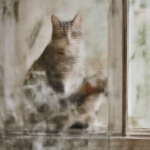 |
 |
 |
These images are blurry but recognizable – the student with teacher weights produces coherent structure in just 4 steps. The KID is 0.069. LADD training should sharpen these images and push KID lower. Instead, it destroyed them.
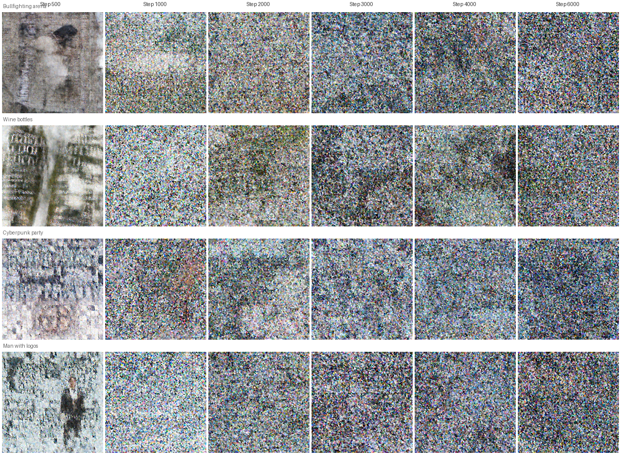
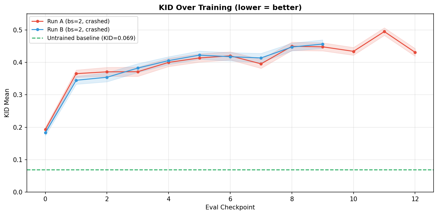
By step 2000, all outputs collapsed into the same colorful noise pattern regardless of prompt. The uniformity across completely different prompts (bullfighting arena, wine bottles, cyberpunk party, watercolor landscape) confirms this is mode collapse, not just poor quality – the student is producing a single “average” output regardless of conditioning. By step 4000, KID reached 0.593 – 8.6x worse than not training at all:
The KID learning curve tells the full story – every checkpoint is worse than the untrained student (green dashed line), and the trend is monotonically upward:
Root cause: config drift
The production run diverged from our validated sweep config in two critical ways:
| Parameter | Production run | Validated best | Impact |
|---|---|---|---|
train_batch_size |
1 | 2-4 | Hinge loss on 1 sample saturates to 0 every micro-step |
renoise_m |
1.0 | 0.5 | Discriminator mostly sees heavily noised samples where gradients are weak |
The combination was lethal: weak gradients from high-noise re-noising (sigmoid(1.0) = 0.73, so the discriminator mostly saw heavily noised samples where real and fake are hard to distinguish), further zeroed out by degenerate hinge loss on single samples. Gradient accumulation across 8 GPUs summed 8 zeros into zero. The student drifted from its teacher-initialized weights into noise with no corrective signal.
The fix was straightforward once diagnosed:
--train_batch_size=2              # was 1 -- hinge loss needs >1 sample
--gradient_accumulation_steps=4   # was 8 -- keeps effective BS=64 (2x4x8)
But by the time we identified the root cause, our compute budget was spent.
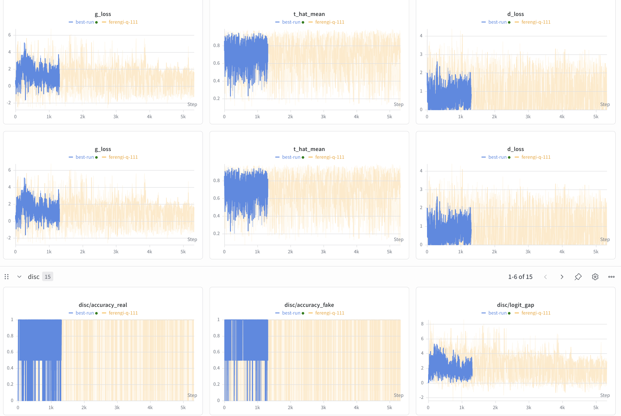
What the metrics showed
The discriminator accuracy metrics told a misleading story: disc/accuracy_real and disc/accuracy_fake both pinned at 1.0 throughout training. This looked like “discriminator too strong, student getting no gradient.” But d_loss and g_loss were actually non-zero and oscillating (0-4 range).
The explanation: accuracy was computed on a per-GPU micro-batch of 1 sample. With bs=1, the discriminator trivially classifies one sample – accuracy can only be 0 or 1. The metric was degenerate, not the training signal itself. The real problem was that the loss was degenerate (hinge loss saturating on single samples), not the accuracy.
This is a broader lesson about adversarial training metrics. Unlike supervised learning where loss monotonically decreases, GAN losses oscillate by design. The question is whether they oscillate healthily. With bs=1, you literally cannot tell from scalar metrics alone whether training is working – you need to look at the generated images.
6. Lessons Learned
Validate your baseline before tuning anything. We ran 21 experiments and found an 89% KID improvement – then discovered 5 critical bugs in the training pipeline: (1) scheduler linspace off-by-one leaving 11% residual noise at the final step, (2) teacher reference images generated without CFG (guidance_scale=0 instead of 5, producing washed-out unconditional-like outputs), (3) student receiving pure noise regardless of timestep ($x_t$ at $t=0.25$ should be mostly clean but was pure static), (4) no velocity-to-latent conversion (using raw velocity instead of $\hat{x}0 = x_t - t \cdot v\theta$), and (5) “real” samples being noise-vs-noise instead of re-noised teacher latents. Every KID number became meaningless – and the optimal GI flipped from 8 to 3 once the discriminator faced a genuinely hard task. Before any sweep, verify the teacher produces sharp images, the training math matches the paper step-by-step, and a single step produces non-trivial gradients. Log teacher outputs to W&B as a sanity check before starting experiments.
Budget compute end-to-end. We curated 500K diverse prompts but could only precompute 10K teacher latents in our compute window (2% of the dataset). At ~7.3s per image across 8 GPUs, all 500K would take 127 hours – we had 6 hours. The 10K subset overfits quickly (KID degrades after 500 steps on 3K data). Model the full pipeline cost – data curation, precomputation, training, and evaluation – before committing to any stage. Our 500K prompts are valuable for future runs, but for the first training run, we should have known the constraint earlier and sized the curation accordingly.
Per-micro-step batch size matters for the loss function. The total effective batch size (bs x GPUs x grad_accum) is not the only thing that matters – the per-GPU batch size determines whether the loss function produces meaningful gradients within each micro-step. Hinge loss with bs=1 is degenerate: ReLU(1 - logit) on a single sample is either exactly 0 (discriminator confident, no gradient) or fully active (max gradient), with no intermediate values. Gradient accumulation sums 8 of these binary values across GPUs, which is better than a single zero but still far worse than a proper batch.
Moving to bs=2 per GPU made loss curves readable and training stable, while keeping the same effective batch size (2 x 8 GPUs x 4 grad_accum = 64) by halving gradient accumulation steps from 8 to 4. The discriminator accuracy metric also became meaningful – with bs=1, accuracy is binary (0 or 1); with bs=2, it can be 0, 0.5, or 1, giving a coarse but real signal.
Log images, not just scalars. Scalars like KID and d_loss tell you that something is wrong; images tell you what. The scheduler bug was caught only because we logged teacher images to W&B as part of a CFG sweep – the images looked blurry at all CFG values, which prompted investigation of the scheduler. The mode collapse was obvious from images at step 2000 but invisible in the loss curves, which oscillated in normal ranges (0-4, exactly where healthy adversarial training should be). At minimum, log: teacher outputs at step 0, student predictions every N steps, the scheduler sigma schedule, and student input $x_t$ at different timesteps. A 5-minute W&B setup saves days of blind debugging.
Debug slices are a different problem than full scale. Our 98-prompt debug slice succeeded because each prompt was seen every ~98 steps – the student cycled through familiar prompts fast enough to mask the degenerate bs=1 dynamics. With rapid prompt cycling, the implicit diversity of seeing many different discriminator judgments in quick succession created enough gradient variety to keep training stable.
At 10K prompts, each prompt appears every ~10K steps, and the bs=1 problem dominates. The student no longer cycles through familiar prompts fast enough to maintain that implicit diversity. Worse, the production config accidentally drifted from the validated sweep config (different renoise_m and warmup_schedule_steps). No automated check caught the mismatch. Always diff your launch command against your sweep winner. An automated config comparison step before launch would have caught this – and we have since added one.
7. What’s Next
Despite the mode collapse on the full run, the architecture and methodology are sound. Single-GPU experiments showed the student learning structure, text conditioning working correctly (compositions matching prompts), and KID improving over the untrained baseline. The student at 2000 steps picked up layout details like bold text, speaker images, and URL placement even on complex advertisement prompts. The bottleneck is compute scale and configuration discipline, not the fundamental approach.
Here is what we would prioritize on the next attempt:
-
More fine-grained evaluation – run KID every 500 steps out to 4000+ to map the full degradation curve and identify the optimal early-stopping point. Our current evaluation was too sparse to catch the collapse early.
-
Higher per-GPU batch size (bs=4+) for more stable gradient flow. Hinge loss quality improves monotonically with batch size. This requires memory optimization (activation checkpointing, gradient offloading) to fit on A100 80GB alongside the 12GB frozen teacher.
-
Alternative loss functions – non-saturating loss, Wasserstein loss, or R1 gradient penalty may provide more stable gradients than hinge loss, especially at small batch sizes where the hinge saturates. R1 penalty in particular is a standard GAN regularizer we haven’t tried.
-
EMA weight updates – maintain a running average of student weights to smooth out oscillations during adversarial training. This is a standard GAN stabilization technique (used in StyleGAN, BigGAN, etc.) that we haven’t explored yet.
-
Scale up training data – precompute latents for 50K+ prompts to reduce overfitting and enable longer training runs. Our 10K subset overfits after ~500 steps; 50K should allow the 20K-step training we originally targeted.
-
Multi-seed averaging – run 3-5 seeds per config and report mean KID to avoid false confidence from lucky single runs. Our variance analysis showed that single-run results can be 2x better than the true mean.
The fundamental tension in LADD is that the discriminator must be strong enough to provide signal but not so strong that it overwhelms the student. Our experiments showed this sweet spot is narrow and sensitive to batch size, learning rate, and update frequency. With better compute budget planning and stricter config management, the next run should avoid the collapse that derailed this one.
8. References
| Year | Paper | Contribution |
|---|---|---|
| 2023 | Lipman et al., Flow Matching for Generative Modeling | Flow matching framework – linear interpolation, velocity prediction |
| 2023 | Sauer et al., Adversarial Diffusion Distillation (ADD) | First adversarial distillation for diffusion – SDXL-Turbo, 1-4 steps |
| 2024 | Sauer et al., LADD: Latent Adversarial Diffusion Distillation | Discrimination in teacher latent space – 14M discriminator for 6B+ models |
| 2018 | Miyato et al., Spectral Normalization for GANs | Hinge loss and spectral norm for stable adversarial training |
| 2018 | Perez et al., FiLM: Visual Reasoning with Feature-wise Linear Modulation | FiLM conditioning used in discriminator heads |
This post is part of a series on distilling Z-Image. Part 1: Data Curation covers how we assembled 500K diverse prompts from 9 sources. Part 2: Training Framework is the full technical deep-dive with all code, W&B screenshots, and debugging details.